CHAPTER 1 Introduction to SPECsfs
Introduction to SPEC SFS 3.0
SPEC SFS 3.0 (SFS97_R1) is
the latest version of the Standard Performance Evaluation Corp.'s benchmark
that measures NFS file server throughput and response time. It provides
a standardized method for comparing performance across different vendor
platforms. This is an incremental release that based upon the design of
SFS 2.0 (SFS97) and address several critical problems uncovered in that release,
additional it addresses several tools issues and revisions to the
run and reporting rules.
The major features of SPEC SFS 3.0 (SFS97_R1) includes:
• resolves defects uncovered in SFS 2.0
• measures results for both NFS protocol version 3 and version 2,
• either TCP or UDP can be used as the network transport,
• the operation mix closely matches real-world NFS workloads,
• the benchmark distribution CD includes precompiled and tested binaries,
• has an interface to accommodate both accomplished and novice users,
• includes report page generation tool.
This document specifies the guideline on how SPEC SFS 3.0 is to be run
for measuring and publicly reporting performance results. These rules
have been established by the SPEC SFS Subcommittee and
approved by the SPEC Open Systems Steering Committee. They ensure that
results generated with this suite are meaningful, comparable to other generated
results, and are repeatable. Per the SPEC license
agreement, all results publicly disclosed must adhere to these Run
and Reporting Rules.
This document also includes the background and design of the SFS benchmark
and a guide to using the SFS tools.
History of SPEC SFS
LADDIS to SPECsfs
SPEC released SFS 1.0 in 1993. In November of 1994 SFS 1.1 was released which fixed a set of minor problems. Version 1.X of the SFS benchmark and its related work load were commonly referred to as LADDIS [Wittle]. SFS 1.X contains support for measuring NFS version 2 servers with the UDP network transport.
With the advance of NFS server technology and the continuing change in customer workloads, SPEC has updated SFS 1.1 to reflect these changes. SFS 2.0, released in December of 1997, reflects the efforts of SPEC in this regard. With the release of SFS 2.0, the LADDIS name was replaced with the preferred name of SPECsfs97.
The old SFS 1.1 work load
The SPECsfs benchmark is a synthetic benchmark that generates an increasing load of NFS operations against the server and measures the response time (which degrades) as load increases. The older version, SFS 1.1, only supports NFS version 2 over UDP for results generation. SFS 2.0 added support for NFS version 3 server measurements. SFS 2.0 also added support for the use of TCP as a network transport in generating benchmark results. The SPECsfs workload consists primarily of the mix of NFS operations, the file set, block size distribution, and the percentage of writes which are appends versus overwrites.
The single workload in SFS 1.1 measured NFS Version 2 over UDP and presented the server with a heavy write-oriented mix of operations (see Table 1).
The 15% WRITE component for NFS was considered high, and WRITE activity dominated processing on most servers during a run of the SFS 1.1 work load. The operation mix for the SFS 1.1 workload was obtained primarily from nhfsstone (a synthetic NFS Version 2 benchmark developed by Legato Systems). Block size and fragment distributions were derived from studies at Digital. Append mode writes accounted for 70% of the total writes generated by the workload.
In SFS 1.1, 5MB per NFS op/s of data was created to force increasing disk head motion when the server misses the cache and 1MB per NFS op/s was actually accessed (that is 20% of the data created was accessed at any point generated). The 1MB of data accessed per NFS op/s was accessed according to a Poisson distribution to provide a simulation of more frequently accessed files.
TABLE 1. SFS work loads and their mix percentages
| NFS |
SFS 1.1 |
SFS 2.0 & 3.0 |
SFS 2.0 & 3.0 |
| Operation |
NFSv2 |
NFSv2 |
NFSv3 |
| LOOKUP |
34% |
36% |
27% |
| READ |
22% |
14% |
18% |
| WRITE |
15% |
7% |
9% |
| GETATTR |
13% |
26% |
11% |
| READLINK |
8% |
7% |
7% |
| READDIR |
3% |
6% |
2% |
| CREATE |
2% |
1% |
1% |
| REMOVE |
1% |
1% |
1% |
| FSSTAT |
1% |
1% |
1% |
| SETATTR |
1% |
||
| READDIRPLUS |
9% |
||
| ACCESS |
7% |
||
| COMMIT |
5% |
The work loads for SFS 2.0
SFS 2.0 supported both NFS version 2 and NFS version 3. The results for each version were not comparable. The NFS Version 2 mix was derived from NFS server data. The NFS Version 3 mix was desk-derived from the NFS Version 2 mix. Neither of these workloads were comparable to the SFS 1.1 work load
Basis for change in mix of operations.
From SFS 1.1, there were two main areas of change in the workload generated by the benchmark. To determine the workload mix, data was collected from over 1000 servers over a one month period. Each server was identified as representing one of a number of environments, MCAD, Software Engineering, etc. A mathematical cluster analysis was performed to identify a correlation between the servers. One cluster contained over 60% of the servers and was the only statistically significant cluster. There was no correlation between this mix and any single identified environment. The conclusion was that the mix is representative of most NFS environments and was used as the basis of the NFS version 2 workload.
Due to the relatively low market penetration of NFS version 3 (compared to NFS version 2), it was difficult to obtain the widespread data to perform a similar data analysis. Starting with the NFS version 2 mix and using published comparisons of NFS version 3 and NFS version 2 given known client workloads [Pawlowski], the NFS version 3 mix was derived and verified against the Sun Microsystems network of servers.
Modifications in the file set in SFS 2.0
The file sets in the SFS 2.0 and workloads were modified so that the overall size doubled as compared to SFS 1.1 (10 MB per ops/s load requested load). As disk capacities have grown, so has the quantity of data stored on the disk. By increasing the overall file set size a more realistic access pattern was achieved. Although the size doubled, the percentage of data accessed was cut in half resulting in the same absolute amount of data accessed. While the amount of disk space used grew at a rapid rate, the amount actually accessed grew at a substantially slower rate. Also the file set was changed to include a broader range of file sizes (see table 2 below). The basis for this modification was a study done of a large AFS distributed file system installation that was at the time being used for a wide range of applications. These applications ranged from classic software development to administrative support applications to automated design applications and their data sets. The SFS2.0 file set included some very large files which are never actually accessed but which affect the distribution of files on disk by virtue of their presence.
The new work loads for SFS 3.0
There is no change in the mix of operations in SFS 3.0. (See TABLE 1 above) The mix is the same as in SFS 2.0. However, t he results for SFS 3.0 are not comparable to results from SFS 2.0 or SFS 1.1. SFS 3.0 contains changes in the working set selection algorithm that fixes errors that were present in the previous versions. The selection algorithm in SFS 3.0 accurately enforces the originally defined working set for SFS 2.0. Also enhancements to the workload mechanism improve the benchmark's ability to maintain a more even load on the SUT during the benchmark. These enhancements affect the workload and the results. Results from SFS 3.0 should only be compared with other results from SFS 3.0.
Modifications in the file set in SFS 3.0
The files selected by SFS 3.0 are on a “best fit” basis, instead of purely random as with SFS 1.1. The “best fit” algorithm in SFS 2.0 contained an error that prevented it from working as intended. This has been corrected in SFS 3.0.
SFS 3.0 contains changes in the working set selection algorithm that fix errors that were present in the previous versions. The file set used in SFS 3.0 is the same file set as was used in SFS 2.0 with algorithmic enhancements to eliminate previous errors in the file-set selection mechanism. The errors in previous versions of SFS often reduced the portion of the file-set actually accessed, which is called the "working set" .
TABLE 2. File size distribution
| Percentage |
Filesize |
| 33% |
1KB |
| 21% |
2KB |
| 13% |
4KB |
| 10% |
8KB |
| 8% |
16KB |
| 5% |
32KB |
| 4% |
64KB |
| 3% |
128KB |
| 2% |
256KB |
| 1% |
1MB |
What is new in SFS 3.0
There are several areas of change in the SPEC SFS 3.0 benchmark. The changes are grouped into the following areas:
• Measurement of time.
• Regulation of the load.
• Working set and file access distribution.
• Other enhancements
• Documentation changes
Within each of these areas there is a brief description of what motivated the change along with a detailed description of the new mechanisms.
Gettimeofday () resolution.
In the SFS 2.0 benchmark time was measured with the gettimeofday () interface. The function gettimeofday () was used to measure intervals of time that were short in duration. SFS 3.0 now measures the resolution of the gettimeofday () function to ensure its resolution is sufficient to measure these short events. If the resolution of gettimeofday () is 100 microseconds or better then the benchmark will proceed. If it is not then the benchmark will log the resolution and terminate. The user must increase the resolution to at least 100 microseconds before the benchmark will permit the measurement to continue.
Select () resolution compensation.
In the SFS benchmark there is a regulation mechanism that establishes a steady workload. This regulation mechanism uses select () to introduce sleep intervals on the clients. This sleep interval is needed if the client is performing more requests than was intended. In SFS 2.0 the regulation mechanism relied on select () to suspend the client for the specified number of microseconds. The last parameter to select is a pointer to a timeval structure. The timeval structure contains a field for seconds and another field for microseconds. The implementation of select may or may not provide microsecond granularity. If the requested value is less than the granularity of the implementation then it is rounded up to the nearest value that is supported by the system. On many systems the granularity is 10 milliseconds. The mechanism in SFS 2.0 could fail if the granularity of the select () call was insufficient. It was possible that the benchmark could attempt to slow the client by a few milliseconds and have the unintended effect of slowing the client by 10 milliseconds or more.
The SFS 2.0 benchmark makes adjustments to the sleep interval at two different times during the benchmark. During the warm-up phase the benchmark makes adjustments every 2 seconds. In the run phase it makes adjustments every 10 seconds. Once the adjustment was made the adjustment value was used for the rest of the interval (2 seconds or 10 seconds) until the next time the adjustment was recalculated. If the granularity of select's timeout was insufficient then the sleep duration would be incorrect and would be used for the entire next interval.
The mechanism used in SFS 3.0 is more complex. The sleep interval is calculated as it was in SFS 2.0. When the client is suspended in select () and re-awakens it checks the amount of time that has passed using a the gettimeofday () interface. This allows the client to know if the amount of time that it was suspended was the desired value. In SFS 3.0 the requested sleep interval is examined with each NFS operation. If the requested sleep interval was for 2 milliseconds and the actual time that the client slept was 10 milliseconds then the remaining 8 milliseconds of extra sleep time is remembered in a compensation variable. When the next NFS operation is requested and goes to apply the sleep interval of 2 milliseconds the remaining 8 milliseconds is decremented by the requested 2 milliseconds and no actual sleep will be performed. Once the remainder has been consumed then the process begins again. This mechanism permits the client to calculate and use sleep intervals that are smaller than the granularity of the select () system call. The new mechanism performs these compensation calculations on every NFS operation.
The gettimeofday() interface measures wall clock interval that the
process was suspended by select (). This interval may occasionally
include periods of time that were unrelated to select (), such
as context swtiches, cron jobs, interrupts, and so on. SFS 3.0 resets
the compensation variable whenever it reaches 100 milliseconds, so that
noise from unrelated events does not overload the compensation mechanism.
Regulation of the workload
The SFS 2.0 benchmark uses a mechanism to establish a steady workload. This mechanism calculates the amount of work that needs to be completed in the next interval. It calculates the amount of sleep time (sleep duration per NFS operation) that will be needed for each operation so that the desired throughput will be achieved. During the warm-up phase the interval for this calculation is every 2 seconds. During the run phase the interval for this calculation is every 10 seconds. If the client performs more operations per second than was desired then the sleep duration for each NFS operation over the next interval is increased. In SFS 2.0 the sleep duration for each NFS operation could be increased too quickly and result in the client sleeping for the entire next. This resulted in no work being performed for the entire next interval. When the next interval completed then the algorithm in SFS 2.0 could determine that it needed to decrease the sleep duration for the next interval. The next interval would perform work and could then again have performed too much work and once again cause the next sleep duration calculation to overshoot and cause the next interval to perform no work. This oscillation could continue for the duration of the test.
In SFS 3.0 the nerw sleep interval is restricted to be no more than:
2 * (previous_sleep_interval +5) Units are in milliseconds
This reduces how aggressively the algorithm increments the sleep interval and permits the steady workload to be achieved. In SFS 2.0 the calculation for how much work to perform in the next interval would attempt to catch up completely in the next interval. This has been changed so that the sleep duration will not change to rapidly.
SFS 3.0 also checks the quantity of work to be performed for each interval, in the run phase, and if any interval contains zero operations then the benchmark logs an error and terminates.
Working set and file distribution
In order to understand the changes in the SFS 3.0 benchmark there is need for the reader to become familiar with several internal mechanisms in SFS 2.0. The following is a brief description of these mechanisms. The following graphic is provided to assist in understanding the overall file distribution of SFS.
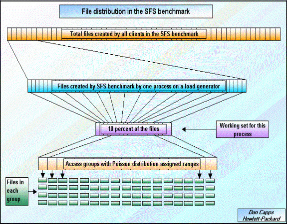
The SFS benchmark creates files that will later be used for measurement of the system's performance. The working set of the SFS benchmark is 10 percent of all of the files that it creates. This working set is established when the benchmark initializes. This initialization groups the files in the working set into access groups. Each group contains the same number of files. For each group there is a probability of access that is calculated using a Poisson distribution for all of the groups. The use of a Poisson distribution simulates the access behavior of file servers. That behavior being that some files are accessed more frequently than others. The Poisson probability is used to create a range value that each group encompasses. The range value for each group is the
Poisson probability * 1000 + previous_groups_range_value. For groups with a low probability the range value is incremented by a small number. For groups with a high probability the range value is incremented by a large number.
During the run phase each NFS operation selects one of the files in the working set to be accessed. Since the time to select the file is inside the measurement section it is critical that the file selection mechanism be as non-intrusive as possible. This selection mechanism uses a random number that is less than or equal to the maximum range value that was calculated for all the groups. A binary search of the group's ranges is performed to select the group that corresponds to this random value. After the group is selected then another random number is used to select a particular file within the group.
The following is a graphical representation of the SFS 2.0 Poisson distribution that would be used when the operations/second/process is 25. This results in 12 access groups with the access distribution seen below.
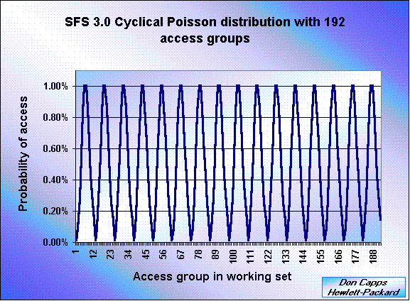
The problem with SFS 2.0 is that the Poisson distribution could deteriorate as the number of files being accessed by any process became large. The probabilities for some of the access groups became zero due to rounding. The following is a graphical representation of the SFS 2.0 Poisson distribution that would be used when the operations/sec/process is increased and there are 192 access groups.

In SFS 2.0 the number of files in the working set is reduced as the number of operations/sec/proc is increased.
The algorithm also contained a mathematical error that could eventually reduce the number of access groups to one. This was not seen in any previous results as the criteria to activate this defect was that the number of operations/second/process would need to be above 500 and no previous results were in this range. For more details on each defect in SFS 2.0 see the “Defects in SFS 2.0” written by Stephen Gold from Network Appliance on the SPEC web site.
The defects in SFS 2.0 resulted in an overall reduction in the working set and may have impacted the SPECsfs97 results. The exact impact on the result depends on the size of the caches in the server and other factors. If the caches were sufficiently large as to encompass the entire 10 percent of all of the files that were created (the intended working set) then the impact on the result may be negligible. This is because if all of the files that should have been accessed would have fit in the caches then the selection of which file to access becomes moot.
In SFS 3.0 the file selection algorithm has been changed so that reduction
of the working set no longer occurs. The algorithm in SFS 3.0 is based
on the Poisson probabilities used in SFS 2.0, but SFS 3.0
manipulates the probabilities to ensure that all of the files in the
working set have a reasonable probability of being accessed.
To achieve this, SFS 3.0 implements a "cyclical Poisson" distribution.
The following graph shows the SFS 3.0 access probabilities for 192 access
groups:
Instead of varying the parameter of the Poisson distribution to generate
values for 192 access groups, the relative probabilities for 25 ops/sec
(12 access groups) are simply repeated as many times as
necessary. Thus there are no access groups with extremely small probabilities,
and no huge floating-point values are needed to compute them.
For 192 access groups, a total of 16 repetitions or "cycles" are
used. Each cycle of access groups has the same aggregate probability of
access, namely 1/16. (The number of access groups in SFS 3.0 is always
a multiple of 12, so there are no partial cycles.)
The Poisson probabilities for 25 ops/sec (12 access groups) are scaled
down by 16 (the number of cycles) and applied to the first 12 access groups,
which constitute the first cycle of the distribution. The same
probabilities are also applied to the next 12 access groups (the second
cycle) and the process is repeated across all 16 cycles.
Another view of the working set is to divide it into 12 distinct access-group "generations",
each of which is represented by a single access group in each cycle. Within
a given generation, all the access-groups have the same probability of
access. For instance, groups 1, 13, 25, ... 181 constitute one generation.
The cache profile across 192 groups looks very much like the cache profile across 12 groups. Why is this the case? The answer is that the cyclical Poisson distribution results in the following distribution of accesses across generations:

In the above graph there are still 192 access groups, but they have been
aggregated together into 12 generations. The probability of access
for each generation has been plotted. Note that the curve for
192 access groups (with 16 access groups per generation) looks the
same as the one for 12 access groups (with one access group per generation).
Hence the cache behavior of SFS is no longer sensitive to the number
of load-generating processes used to achieve a given request rate.
In theory, the same effect could have been achieved by always having
12 access groups, no matter how many files there are. This was not
done for fear that exhaustive searches for files within a very large access
group would be expensive, causing the load-generators to bog down in
file selection.
Other changes in SFS 3.0
Support for Linux & BSD clients
The SFS 3.0 benchmark contains support for Linux and BSD clients. As the popularity of these other operating systems continues to grow the demand for their support was seen as an indication of the importance of SFS support.
Best fit algorithm
In SFS 2.0 after a access group was selected for access, a file was selected for access. This selection was done by picking a random file within the group to be accessed and then searching for a file that meets the transfer size criteria. There was an attempt to pick a file based on the best fit of transfer size and available file sizes. This mechanism was not working correctly due to an extra line of code that was not needed. This defect resulted in the first file to have a size equal to or larger than the transfer size being picked.
SFS 3.0 eliminates the extra line of code and permits the selection to be a best fit selection instead of a first fit selection.
New submission tools
The “generate” script is now included with SFS 3.0. This shell script is used to create the submission that is sent to SPEC for review and publication of SFS results.
Readdirplus() enhancements.
In SFS 2.0 the benchmark tested the Readdirplus() functionality of NFS version 3. However it did not validate that all of the requested data was returned by the operation. SFS 3.0 performs the additional validation and ensures that all of the requested attributes and data are returned from the Readdirplus() operation.
Minor changes.
Updated release number from 2.0 to 3.0.
Updated version date from " 23 October 1997 " to " 20
June 2001 ".
Updated all SPEC copyrights to 2001.
Update SPEC mailing address to reflect move from Manassas
to Warrenton.
Reduction in the memory required by each client to run the benchmark.
Bug fixes.
Corrected the calculations of atime.nseconds
and mtime.nseconds.
Format total_fss_bytes using "%10lu" instread
of "%10d" to avoid wraparound.
Set variables in sfs_mcr so that processes
get cleaned up.
Fix a typo in the sample sfs_rc.
Source and build changes for portability
New compiler flags for IBM.
Add "linux" and "freebsd" wrappers.
Don't include <stropts.h> on FreeBSD.
Save sockaddr_in before calling ioctl(SIOCGIFFLAGS).
Limit select's size to FD_SETSIZE.
Remove unused svc_getreq() function which
was nonportable.
Shell-script changes for portability
Implemented a better way to set CDROM_BENCHDIR.
Removed use of the "function" keyword
when defining shell functions.
Deleted dangling "-a" in installsfs
conditional.
Added missing back-tics in install_sfs and
run_sfs.
Eliminated dependencies on /usr/tmp directory.
Use back-tic to set SPEC_HOME.
Don't use '.' to invoke sfsenv.
Use pwd_mkdb to update FreeBSD password database.
Documentation changes in SFS 3.0
The SFS 3.0 Users Guide has been updated to reflect:
- The changes in the benchmark
- The new supported clients
- Changes in the run rules
- Addition of information on submission tools.
- Changes in the disclosure rules.
- Documentation is now in HTML, rich text, and PDF formats for portability.
CHAPTER 2 Running Instructions
Detailed Running Instructions
Configuration
There are several things you must set up on your server before you can successfully execute a benchmark run.
1. Configure enough disk space. SPECsfs needs 10 MB of disk space for each NFSops you will be generating, with space for 10% growth during a typical benchmark run (10 measured load levels, 5 minutes per measured load). You may mount your test disks anywhere in your server's file space that is convenient for you. The NFSops a server can process is often limited by the number if independent disk drives configured on the server. In the past, a disk drive could generally sustain on the order of 100-200 NFSops. This was only a rule of thumb, and this value will change as new technologies become available. However, you will need to ensure you have sufficient disks configured to sustain the load you intend to measure.
2. Initialize and mount all file systems. According to the Run and Disclosure Rules, you must completely initialize all file systems you will be measuring before every benchmark run. On Unix systems, this is accomplished with the “newfs” command. Just deleting all files on the test disks in not sufficient because there can be lingering effects of the old files (e.g. the size of directory files, location of inodes on the disk) which effect the performance of the server. The only way to ensure a repeatable measurement is to re-initialize all data structures on the disks between benchmark runs. However, if you are not planning on disclosing the result, you do not need to perform this step.
3. Export all file systems to all clients. This gives the clients permission to mount, read, and write to your test disks. The benchmark program will fail without this permission.
4. Verify that all RPC services work. The benchmark programs use port mapping, mount, and NFS services provided by the server. The benchmark will fail if these services do not work for all clients on all networks. If your client systems have NFS client software installed, one easy way to do this is to attempt mounting one or more of the server's disks on the client. NFS servers generally allow you to tune the number of resources to handle UDP and/or TCP requests. When benchmarking using the TCP protocol , you must make sure that UDP support is at least minimally configured or the benchmark will fail to initialize.
5. Ensure your server is idle. Any other work being performed by your server is likely to perturb the measured throughput and response time. The only safe way to make a repeatable measurement is to stop all non-benchmark related processing on your server during the benchmark run.
6. Ensure that your test network is idle. Any extra traffic on your network will make it difficult to reproduce your results, and will probably make your server look slower. The easiest thing to do is to have a separate, isolated network between the clients and the server during the test.
At this point, your server should be ready to measure. You must now set up a few things on your client systems so they can run the benchmark programs.
1. Create “spec” user. SPECsfs should run as a non-root user.
2. The SPECsfs programs must be installed on clients.
3. Ensure sfs and sfs3 are setUID root, if necessary. Some NFS servers only accept mount requests if sent from a reserved UDP or TCP port, and only the root user can send packets from reserved ports. Since SPECsfs generally is run as a non-root user, the sfs and sfs3 programs must be set to execute with an effective UID of root.
To get the benchmark to use a reserved port, you must include a -DRESVPORT option in your compile command. This is easiest to accomplish by editing the Makefile wrapper file (M.xxxx) for your client systems. The build process will then make the client use a reserved port and will arrange to run the benchmark programs as root. However, you may want to verify this works the first time you try it.
4. Configure and verify network connectivity between all clients and server. Clients must be able to send IP packets to each other and to the server. How you configure this is system-specific and is not described in this document. Two easy ways to verify network connectivity are to use a “ping” program or the netperf benchmark (http:// onet1.external.hp.com/netperf/NetperfPage.html) .
5. If clients have NFS client code, verify they can mount and access server file systems. This is another good way to verify your network is properly configured. You should unmount the server's test disks before running the benchmark.
6. Configure remote shell access. The Prime Client needs to be able to execute commands on the other client systems using rsh (remsh on HP-UX, AT&T Unix, and Unicos). For this to work, you need to create a .rhosts file in the spec user's home directory.
A good test of this is to execute this command from the prime client:
$ rsh client_name "rsh prime_client date"
If this works, all is well.
7. The Prime Client must have sufficient file space in the SFS file tree to hold the result and log files for a run. Each run generates a log file of 10 to 100 kilobytes, plus a result file of 10 to 100 kilobytes. Each client also generates a log file of one to 10 kilobytes.
Once you have the clients and server configured, you must set some parameters for the benchmark itself, which you do in a file called the “rc file”. The actual name of the file is a prefix picked by you, and the suffix “_rc”. The default version shipped with the benchmark is delivered as “sfs_rc” in the benchmark source directory. The SPECsfs tools allow you to modify parameters in the rc file. If you want to manually edit this file, the sfs_rc file should be copied to the results directory. The sfs_rc file can then be edited directly. The sfs_rc file is executed by a Bourne shell program, so all the lines in the RC file must be in Bourne shell format. Most important, any variable which is a list of values must have its value enclosed in double quotes.
There are several parameters you must set, and several others you may change to suit your needs while performing a disclosable run. There are also many other parameters you may change which change the benchmark behavior, but lead to an undisclosable run (for example, turning on debug logging).
The parameters you can/must set are:
1. MNT_POINTS : This parameter specifies the names of the file systems the clients will use when testing the server. It can take two forms.
The first form is a list of host:path pairs specifying the file systems this particular client will be using. For example, if the server is named “testsys” and has three test mount points named “/test1”, “/test2”, and “/test3”, the list would be “testsys:/test1 testsys:/test2 testsys:/test3”. You must be very careful when specifying the mount point to comply with the uniform access rule (see below).
The second form is simply the name of a file containing a list of mount points for each client. The format of the file is:
client_name server:path server:path...
client_name server:path server:path...
And so on, one line for each client system. This file gets stored in the “results” directory, the same place as the rc file.
2. LOAD , INCR_LOAD , and NUM_RUNS : These parameters specify the aggregate load the clients will generate. You can specify the load points two ways:
• You can explicitly specify a list of load levels in LOAD. So, if you want to test a load of 100, 300, and 700 NFSops, you would set LOAD to “100 300 700".
• If you want to test a set of evenly spaced load points, set all three parameters. Set LOAD to the lowest load level, set INCR_LOAD the amount you would like to increase the load for each measured run, and set NUM_RUNS to the number of times you would like to increment the load. This is the easiest way to configure a disclosable run.
For example, if you would like to measure 10 evenly spaced points ending at 2000 NFSops, you would set LOAD to 200, INCR_LOAD to 200, and NUM_RUNS to 10.
3. CLIENTS : This is the names of all the client systems you will use to load your server. If you will be generating load with the prime client, include it on this list.
4. NUM_PROCS : This is the number of load generating processes (“procs”) you want to run on each client system. As you add procs, you can have more NFS requests outstanding at any given time, and you can use more file systems on the server, all of which tends to increase the load your server can process (until either the disks or the processors run out of capacity).
There is a relationship between the value of PROCS, CLIENTS and MNT_POINTS. The number of mount points specified in MNT_POINTS must equal the value of PROCS, or equal the value of PROCS times the number of clients in CLIENTS. In the first case, each mount point will be accessed by one proc on each client. In the second case, each listed mount point will be accessed by exactly one proc on one client. The first PROC mount points will be used by the first client, the second PROC mount points by the second client, and so forth.
You may specify the same mount point multiple times in MNT_POINTS. This allows you to have more than one process accessing a given filesystem on the server, without having all clients loading that filesystem. If a fileystem traverses multiple disks, (Example RAID Level 0, 1 …), then care must be taken to conform to the uniform access rule.
5. NFS_VERSION : This may be left unset or set to 2 to measure NFS protocol version 2, and set to 3 to measure NFS protocol version 3.
6. TCP : Set this to 1 or “on” to use TCP to communicate between the clients and the server. Leave it unset or set to 0 to use UDP.
7. BIOD_MAX_READS and BIOD_MAX_WRITES : SPECsfs emulates the read-ahead and write-behind behavior of NFS block I/O daemons. These allow a client to have multiple read and write requests outstanding at a given time. BIOD_MAX_READS and BIOD_MAX_WRITES configure how many read or write operations SPECsfs will transmit before stopping and waiting for replies. You can set these to any value from 0 to 32, inclusive.
There are many other parameters you can modify in the rc file, but generally none are necessary. They allow you to change the NFS operation mix, change run duration parameters, or turn on debugging information. Modifying most of these parameters will lead to an invalid (that is, undisclosable) run. The full list of parameters is documented at the end of the sfs_rc file and at the end of this section.
Complying with the Uniform Access Rule
The most common way to perform an un-disclose-able run is to violate the uniform access rule See “ SPEC's Description of Uniform Access for SFS 3.0 ” . In some systems, it is possible to complete an NFS operation especially fast if the request is made through one network interface and the data is stored on just the right file system. The intent of the rule is to prevent the benchmarker (that's you) from taking advantage of these fast paths to get an artificially good result.
The specific wording of the rule states that “for every network, all file systems should be accessed by all clients uniformly.” The practical implication of the uniform access rule is you must be very careful with the order in which you specify mount points in the MNT_POINTS variable.
The fool-proof way to comply with the uniform access rule is to have every client access every file system, evenly spreading the load across the network paths between the client and server. This works pretty well for small systems, but may require more procs per client than you want to use when testing large servers.
If you want to run fewer procs on your clients' than you have file systems, you will need to take some care figuring out the mount points for each client.
Uniform access is a slippery subject. It is much easier to examine a configuration and say whether it is uniform than it is to come up with a perfect algorithm for generating complying mount point lists. There will always be new configurations invented which do not fit any of the examples described below. You must always examine the access patterns and verify there is nothing new and innovative about your systems which makes it accidentally violate the uniform access rule.
Below are some examples of generating mount point lists which do comply with the uniform access rule.
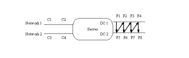
To begin, you must first determine the number of file systems, clients, and load generating processes you will be using. Once you have that, you can start deciding how to assign procs to file systems. As a first example, we will use the following file server:
Clients C1 and C2 are attached to Network1, and the server's address on that net is S1. It has two disk controllers (DC1 and DC2), with four file systems attached to each controller (F1 through F8).

You start by assigning F1 to proc1 on client 1. That was the easy part.
You next switch to DC2 and pick the first unused file system (F5). Assign this to client 1, proc 2.
Continue assigning file systems to client 1, each time switching to a different disk controller and picking the next unused disk on that controller, until client 1 has PROC file systems. In the picture above, you will be following a zig-zag pattern from the top row to the bottom, then up to the top again. If you had three controllers, you would hit the top, then middle, then bottom controller, then move back to the top again. When you run out of file systems on a single controller, go back and start reusing them, starting from the first one.
Now that client 1 has all its file systems, pick the next controller and unused file system (just like before) and assign this to client 2. Keep assigning file systems to client 2 until it also has PROC file systems.
If there were a third client, you would keep assigning it file systems, like you did for client 2.
If you look at the result in tabular form, it looks something like this (assuming 4 procs per client):
C1: S1:F1 S1:F5 S1:F2 S1:F6
C2: S1:F3 S1:F7 S1:F4 S1:F8
The above form is how you would specify the mount points in a file. If you wanted to specify the mount points in the RC file directly, then it would look like this:
CLIENTS=”C1 C2”
PROCS=4
MNT_POINTS=”S1:F1 S1:F5 S1:F2 S1:F6 S1:F3 S1:F7 S1:F4 S1:F8
If we had 6 procs per client, it would look like this:
C1: S1:F1 S1:F5 S1:F2 S1:F6 S1:F3 S1:F7
C2: S1:F4 S1:F8 S1:F1 S1:F5 S1:F2 S1:F6
Note that file systems F1, F2, F5, and F6 each get loaded by two procs (one from each client) and the remainder get loaded by one proc each. Given the total number of procs, this is as uniform as possible. In a real benchmark configuration, it is rarely useful to have an unequal load on a given disk, but there might be some reasons this makes sense.
The next wrinkle comes if you should have more than one network interface on your server, like so:
Clients C1 and C2 are on Network1, and the server's address is S1. Clients C3 and C4 are on Network2, and the server's address is S2.
We start with the same way, assigning F1 to proc 1 of C1, then assigning file systems to C1 by rotating through the disk controllers and file systems. When C1 has PROC file systems, we then switch to the next client on the same network, and continue assigning file systems. When all clients on that network have file systems, switch to the first client on the next network, and keep going. Assuming two procs per client, the result is:
C1: S1:F1 S1:F5
C2: S1:F2 S1:F6
C3: S2:F3 S2:F7
C4: S2:F4 S2:F8
And the mount point list is:
MNT_POINTS=”S1:F1 S1:F5 S1:F3 S1:F7 S2:F2 S2:F6 S2:F4 S2:F8”
The first two mount points are for C1, the second two for C2, and so forth.
These examples are meant to be only that, examples. There are more complicated configurations which will require you to spend some time analyzing the configuration and assuring yourself (and possibly SPEC) that you have achieved uniform access. You need to examine each component in your system and answer the question “is the load seen by this component coming uniformly from all the upstream components, and is it being passed along in a uniform manner to the downstream ones?” If the answer is yes, then you are probably in compliance.
More obscure variables in the RC file.
As mentioned above, there are many more parameters you can set in the RC file. Here is the list and what they do.
The following options may be set and still yield a disclose-able benchmark run:
1. SFS_USER : This is the user name of the user running the benchmark. It is used when executing remote shell commands on other clients from the prime client. You would only want to modify this if you are having trouble remotely executing commands.
2. SFS_DIR and WORK_DIR : These are the directory names containing the SPECsfs programs ( SFS_DIR ), the RC file, and logging and output files ( WORK_DIR ). If you configure your clients with the same path for these directories on all clients, you should not need to fool with this. One easy way to accomplish this is to export the SFS directory tree from the prime client and NFS mount it at the same place on all clients.
3. PRIME_MON_SCRIPT and PRIME_MON_ARGS : This is the name (and argument list) of a program which SPECsfs will start running during the measurement phase of the benchmark. This is often used to start some performance measurement program while the benchmark is running so you can figure out what is going on and tune your system.
Look at the script “sfs_ext_mon” in the SPECsfs source directory for an example of a monitor script.
4. RSH : This is the name of the remote command execution command on your system. The command wrapper file (C.xxxx) should have set this for you, but you can override it here. On most Unix systems, it is “rsh”, but a few (e.g. HP-UX and Unicos), it's called “remsh”.
These remaining parameters may be set, but SPEC will reject the result for disclosure. They are available only to help you debug or experiment with your server
5. WARMUP_TIME and RUNTIME : These set the duration of the warmup period and the actual measurement period of the benchmark. They must be 300, or the submission will be rejected for disclosure.
6. MIXFILE : This specifies the name of a file in WORK_DIR which describes the operation mix to be executed by the benchmark. You must leave this unspecified to disclose the result. However, if you want to change the mix for some reason, this gives you the ability.
Look in the file sfs_c_man.c near the function setmix() for a description of the mix file format. The easiest to use format is as follows:
SFS MIXFILE VERSION 2
opname xx%
opname yy%
# comment
opname xx%
The first line must be the exact string “SFS MIXFILE VERSION 2" and nothing else. The subsequent lines are either comments (denoted with a hash character in the first column) or the name of an operation and it's percentage in the mix (one to three digits, followed by a percent character). The operation names are: null, getattr, setattr, root, lookup, readlink, read, wrcache, write, create, remove, rename, link, symlink, mkdir, rmdir, readdir, fsstat, access, commit, fsinfo, mknod, pathconf, and readdirplus. The total percentages must add up to 100 percent.
7. ACCESS_PCNT : This sets the percentage of the files created on the server which will be accessed for I/O operations (i.e. will be read or written). The must be left unmodified for a result to be submitted for publication.
8. DEBUG : This turns on debugging messages to help you understand why the benchmark is not working. The syntax is a list of comma-separated values or ranges, turning on debugging flags. A range is specified as a low value, a hyphen, and a high value (e.g. “3-5” turns on flags 3, 4, and 5), so the value “3,4,8-10” turns on flags 3, 4, 8, 9, and 10.
To truly understand what gets reported with each debugging flag, you need to read the source code. The messages are terse, cryptic, and not meaningful without really understanding what the code is trying to do. Note the child debugging information will only be generated by one child process, the first child on the first client system. This must not be modified for a valid submission.
Table 3. Available values for the DEBUG flags:
| Value |
Name of flag |
Comment |
| 1 |
DEBUG_NEW_CODE | Obsolete and unused |
| 2 |
DEBUG_PARENT_GENERAL | Information about the parent process running on each client system. |
| 3 |
DEBUG_PARENT_SIGNAL | Information about signals between the parent process and child processes |
| 4 |
DEBUG_CHILD_ERROR | Information about failed NFS operations |
| 5 |
DEBUG_CHILD_SIGNAL | Information about signals received by the child processes |
| 6 |
DEBUG_CHILD_XPOINT | Every 10 seconds, the benchmark checks it's progress versus how well it's supposed to be doing (for example, verifying it is hitting the intended operation rate). This option gives you information about each checkpoint |
| 7 |
DEBUG_CHILD_GENERAL | Information about the child in general |
| 8 |
DEBUG_CHILD_OPS | Information about operation starts, stops, and failures |
| 9 |
DEBUG_CHILD_FILES | Information about what files the child is accessing |
| 10 |
DEBUG_CHILD_RPC | Information about the actual RPCs generated and completed by the child |
| 11 |
DEBUG_CHILD_TIMING | Information about the amount of time a child process spends sleeping to pace itself |
| 12 |
DEBUG_CHILD_SETUP | Information about the files, directories, and mix percentages used by a child process |
| 13 |
DEBUG_CHILD_FIT | Information about the child's algorithm to find files of the appropriate size for a given operation |
Tuning
The following are things that one may wish to adjust to obtain the maximum throughput for the SUT.
- Disks per SFS NFSops
- Networks per SFS NFSops
- Client systems per network
- Memory allocated to buffer cache.
CHAPTER 3 SFS tools
SFS Tools Introduction
This section briefly describes the usage of the run tools provided with the SPEC System File Server (SFS) Release 3.0 suite. These tools provide both a novice mode (query driven) and a advanced mode (menu driven) interface that provide the user with helpful scripts that can set up the environment, set various benchmark parameters, compile the benchmark, conduct benchmark validation, execute the benchmark, view results from a run and archive the results. The results obtained from multiple data points within a run are also collected in a form amenable for ease of use with other result formatting tools. These tools are used on the primary load generator (Prime-Client) for benchmark setup and control as well as on the rest of the NFS load generators (clients) to assist in compiling the programs.
While not required to run the benchmark, the SFS tools can facilitate the “quick” running of the benchmark for tuning various components of the system and results reporting.
This section does not cover the complete Client-Server environment setup in detail. It touches only the portions currently handled by the tools. For information on how to set up and run the SFS suite the reader is advised to refer to the section on running SFS above.
SFS structure
The SFS Benchmark uses the UNIX “Makefile” structure (similar to other SPEC Suites) to build tools, compile the benchmark source into executables, and to clean directories of all executables. If you are familiar with other SPEC suites, navigating around SFS should be very similar. It is important to note that unlike other SPEC benchmarks, SPECsfs's validation and execution functions are built into the “sfs_mgr” script supplied with the benchmark. This script is used by the menu tools when validate or run targets are chosen.
The following is a quick overview of the benchmark's directory structure. Please note that $SPEC is the path in the file system at which the benchmark is loaded.
1. Benchmark tools
The benchmark tools located in the “$SPEC/benchspec/162.nfsv2/src” directory. These tools must be built (as described in the next section) before they can be used. During the tools build, the executables are transferred to the “$SPEC/benchspec/162.nfsv2/ bin”directory.
2. Makefile Wrappers (M.<vendor>)
The Makefile wrappers are located in the “$SPEC/benchspec/162.nfsv2/M.<vendor>” directory. The Makefile wrappers contain specific vendor compiler options and flags.
3. Command Wrappers (C.<vendor>)
The Command wrappers are located in the “$SPEC/benchspec/162.nfsv2/ C.<vendor.>) directory. The Command Wrappers contain the vendor specific command paths and commands for the remote utilities.
4. SPECsfs source
The benchmark source programs are located in the “$SPEC/benchspec/162.nfsv2/src” directory.
5. SPECsfs executables and scripts
Once SPECsfs is compiled, the resultant executables, along with copies of the necessary scripts, are moved to the “$SPEC/benchspec/162.nfsv2/result” directory. This directory is also known as $RESULTDIR.
6. SFS_RC files
Both the SFS default and user modified _rc files are located in the “$SPEC/benchspec/162.nfsv2/result” directory. these files contain the parameter values to be used by the SFS manager (sfs_mgr) script as well as the tools driving the various menus.
Setting up the SFS Environment and building tools
After extracting the SPECsfs suite from the CD, change directory into the uppermost SPEC directory (SPEC home directory). The user's home environment can be initialized by executing:
For C-shell users: “source sfsenv”
For Bourne or Korn shell users: “.
./sfsenv”
By executing this command, the SPEC environment variables SPEC, BENCH, RESULTDIR, TESTSRESULTS, etc. are all defined. The SPEC home directory can now be referenced as $SPEC.
After setting up the SPEC home environment, the tools used by all the menus can be created by the following command:
“make bindir”
Once the make command completes, the “runsfs” script can be used to complete the installation process, to run the benchmark and to view or archive the results.
The “runsfs” script will initially check to see if the sfsenv script has been executed. If it has not, it will execute it. It is important to note that if “runsfs” executes the script, upon exiting the “runsfs” script, environment variables will no longer be set. Additionally, the script will check if the “bindir” directory has been created. If it does not exist, it will create it.
Using the RUNSFS script
The SPECsfs tools consist of a series of scripts that help the user in the installation, configuration, and execution of the benchmark. To invoke these tools, the user should run the “runsfs” script in the $SPEC directory. If the user has not yet executed the “sfsenv” script or created the tools, this script will execute them. The user will initially be prompted for the clients appropriate vendor type.
Example of Vendor Type Prompt
The benchmark has been ported to the following vendor/OS list:
att compaq dec_unix dgc
hpux10 hpux11 ibm ingr
Linux moto sgi sni
solaris2 sunos4 unicos unisys
unixware vendor xpg4.2 freebsd
Please enter your vendor type from the above list or press Return:
dec_unix
The default command file is being set to C.dec_unix .
Executing the C.dec_unix file...
Following the users response, the associated Makefile wrapper and Command wrapper are selected as the default wrappers. If the user wants to skip this step and go directly to the main SFS tools area, they may execute the “run_sfs” script in the “$SPEC/benchspec/162.nfsv2” directory. In this case, the generic Makefile wrapper and Command wrapper (M.vendor and C.vendor) files will be set as the default wrappers.
The user is then prompted if they want to use the Novice User Mode (query driven) or the Advanced User Mode (menu driven). The Novice User Mode is the default session type. This is intended to walk the new user through a benchmark setup, compilation, and execution as well as easily displaying benchmark results. For those familiar with the benchmark's setup and execution, Advanced Mode is preferred.
Example of Preferred Session Type Prompt
SPEC SFS tools may be run in one of two modes
- Novice mode ( query driven )
- Advanced mode ( menu driven )Do you want to run in Advanced mode or Novice mode (a/n(default) )?
Novice Mode
The following selection will summarize the Novice Mode user tools. The Novice Tools assumes that the user is unfamiliar with the SPECsfs environment. The user is led through the test configuration and execution process via a question and answer session. The tools initially help the user setup the client's environment/compiler variables via M.vendor and C.vendor files. After setting up the user environment, the tools allow the user to compile the benchmark, modify the test parameters in the _rc file, run a test, view the results of a test or archive test results. Please note that the
Novice Tools contain a subset of the functions contained in the Advanced Tools.
The following section is intended to present the various functions available to the user via the Novice User Tools. The following examples show the querying structure of the Novice Mode Tools.
Setting the Environment/Compiler Variables
The first series of questions the user must answer deal with selecting the appropriate wrapper files for the particular client/server environment. There are two types of wrapper files, Makefile wrappers and Command Wrappers. The Makefile wrappers contain specific vendor compiler options and flags needed during the compilation process. The Command wrappers contain the vendor specific command paths and commands needed for the remote utilities. This is asked initially, since prior to many of the functions (i.e. benchmark compilation) it is important for the user to select the appropriate wrappers.
Makefile Wrappers
Makefile wrapper selection and compilation of the benchmark programs need to be done on all clients including the Prime-Client after initially installing SPECsfs on the load generators. The user is initially asked if they want to use the default M.vendor file or a different makefile wrapper file.
Do you want to use the default M.vendor file - M.dec_unix
( (y)es, (n)o )?
The default M.vendor file is associated with the client vendor type previously selected. For example, in the previous example, the M.dec_unix file would be selected since a Digital client vendor type was selected. If the default M.vendor file is selected, the user is given the option of modifying its contents. If the user would like to modify the file, the tools will display the contents of the default M.vendor file.
Do you want to use the default M.vendor file - M.dec_unix
( (y)es, (n)o )? yDo you want to edit the M.dec_unix file ((y)es, (n)o)? y
Checking Wrapper file.......
To Continue Please Press The <RETURN> key:
Current Settings
1) MACHID -> dec_osf
2) C COMPILER -> /bin/cc
3) C OPTIONS -> -O
4) C FLAGS ->
5) LOAD FLAGS ->
6) EXTRA CFLAGS -> -DUSE_POSIX_SIGNALS
7) EXTRA LDFLAGS ->
8) LIBS -> -lm
9) EXTRA LIBS ->
10) OSTYPE -> -DOSF1
11) RESVPORT_MOUNT ->
12) Shell Escape
13) Save Wrapper File
14) Return to Main MenuSelect Setting :
If the user would like to use a different M.vendor file, the tool will display a list of all vendor specific makefile wrappers currently available on the CD. The user can look into any vendor wrapper file and modify it suitably and store the file on the system under the same or a different name and use it to compile the benchmark programs. These wrappers are all named with a “M.” prefix.
Do you want to use the default M.vendor file - M.dec_unix
( (y)es, (n)o )? nThe current M.vendor file is: M.dec_unix
--------------------------------------
The following is a list of the available M.vendor wrapper files.
----------------------------------------------------------------
att compaq dec_unix dgc freebsd
hpux10 hpux11 ibm ingr linux
moto sgi sni solaris2
sunos4 unicos unisys unixware
vendor xpg4.2
Enter only the VENDOR part of M.vendor file name
Hit Return if using the current M.dec_unix: hpux11
Checking Wrapper file .......
To Continue Please Press The <RETURN> key:
Current Settings
1) MACHID -> hp
2) C COMPILER -> /opt/ansic/bin/cc
3) C OPTIONS -> -O -Ae
4) C FLAGS -> -D_HPUX_SOURCE
5) LOAD FLAGS ->
6) EXTRA CFLAGS -> -DHAS_GETHOSTNAME -DDNO_T_TYPES
7) EXTRA LDFLAGS ->
8) LIBS -> -lm
9) EXTRA LIBS ->
10) OSTYPE -> -DHPUX
11) RESVPORT_MOUNT ->
12) Shell Escape
13) Save Wrapper File
14) Return to Main MenuSelect Setting :
Note that each item in the above menu is user definable and it is good practice to “save” the wrapper file under a different name if any parameter is modified.
Command Wrappers
The user is then prompted for the appropriate command wrappers (C.vendor) in order to define the appropriate commands and command paths. Users are given the choice of the default C.vendor file or a different command wrapper file.
Do you want to use the default C.vendor file - C.dec_unix
( (y)es, (n)o )?
Similar to the M.vendor files, the default C.vendor file is associated with the client vendor type previously selected. If the user selects the default C.vendor file, they will be given the option to modify the contents of this file. If they would like to modify the file, the tools will display the contents of the c.vendor file.
Do you want to use the default C.vendor command file - C.dec_unix
( (y)es, (n)o, (p)revious )? yDo you want to edit the file ((y)es, (n)o, (p)revious)? y
Current C.vendor Parameter Settings
1) PASSWD_FILE -> /etc/passwd
2) FSTAB_FILE -> /etc/fstab
3) GROUP_FILE -> /etc/group
4) HOSTNAME_CMD -> hostname
5) RSH_CMD -> rsh
6) SHELL -> /bin/sh
7) AWK_CMD -> awk
8) PS_CMD -> ps ax
9) ECHO -> echo
10) NONL ->
11) Shell Escape
12) Save C.vendor File
13) Return to Main MenuSelect Setting :
If the user would like to use a different C.vendor file, the tool will display a list of all vendor specific command wrappers currently available on the CD. The user can look into any vendor wrapper file and modify it suitably and store the file on the system under the same or a different name and use it to compile the benchmark programs. These wrappers are all named with a “C.” prefix.
Do you want to use the default C.vendor command file - C.dec_unix
( (y)es, (n)o, (p)revious )? nThe following is a list of the available C.vendor wrapper files.
----------------------------------------------------------------
C.sgi C.hpux10 C.hpux11 C.sni C.dec_unix freebsd
C.unixware C.vendor C.unicos C.solaris2
C.sunos4 C.intel C.hpux9 C.ibm C.linux C.att
Enter only vendor part of M.vendor File name
Hit Return if using C.dec_unix:
Current C.vendor Parameter Settings
1) PASSWD_FILE -> /etc/passwd
2) FSTAB_FILE -> /etc/fstab
3) GROUP_FILE -> /etc/group
4) HOSTNAME_CMD -> hostname
5) RSH_CMD -> rsh
6) SHELL -> /bin/sh
7) AWK_CMD -> awk
8) PS_CMD -> ps ax
9) ECHO -> echo
10) NONL ->
11) Shell Escape
12) Save C.vendor File13) Return to Main Menu
Select Setting :
Note that each item in the above menu is user definable and it is good practice to “save” the wrapper file under a different name if any parameter is modified.
Once the environment setup is complete, the user enters the main execution loop. The main execution loop is:
Enter whether you want to (r)un, re(c)ompile, (e)dit an .rc file,
(v)iew results, (a)rchive results, (p)revious question, (q)uit ...
The user is now given the option to: run the benchmark: compile (or recompile) the benchmark, edit the _rc file, view existing test results, archive test results, or quit the test.
Running the Benchmark
I
If the user selects the run option, the tools will check if the benchmark has been compiled previously. If it has not yet been compiled, the tools will initially compile the benchmark.
Enter whether you want to (r)un, re(c)ompile, (e)dit an .rc file,
(v)iew results, (a)rchive results, (p)revious question, (q)uit ... rExecutable not found ... compiling benchmark ...
The current M.vendor file is: M.dec_unix
--------------------------------------
The following is a list of the available M.vendor wrapper files.
----------------------------------------------------------------
att compaq dec_unix dgc
hpux10 hpux11 ibm ingr
linux moto sgi sni solaris2
sunos4 unicos unisys unixware
vendor xpg4.2
Enter only the VENDOR part of M.vendor file name
Hit Return if using the current M.dec_unix:
chmod +x run_sfs
`librpclib.a' is up to date.
:
:
:
./sfs_suchown sfs sfs3
... Done
To Continue Please Press The <RETURN> key:
Once there is a benchmark executable available, the user will then be prompted for the appropriate _rc file. The user is then allowed to select the appropriate _rc file. The user may select from any existing _rc files or may create a new file.
List of Available RC Files that End with _rc - Latest First
---------------------------------------------------------------------
don_rc short_v2_rao_2dsk_rc stephen_tcp_v3_rc test_tcp_2_rc
augie_tcp_3_rc test_tcp_v2_rc test_tcp_v3_rc test_udp_2_rc
debug_tcp_2_rc full_tcp_v2_rc full_tcp_v3_rc full_udp_v2_rc
full_udp_v3_rc remote_rc sfs_rc short_rc
short_tcp_rc short_udp_v3_rc temp_rc test_new_rcEnter your RC File name
Hit Return if using original sfs_rc templates with
default values. This will prompt you for new
for new parameter values.Else pick up an existing “ _rc” file from above list:
If the user selects the option to create a new _rc file using the sfs_rc file, they will be prompted for the appropriate parameter values
Load information:
-----------------Current value of LOAD Inital/Series:
To retain this value type <RETURN>
For null value type <space> & <RETURN>
The requested load is the total load applied to the server.
Example of a full curve: 100 200 300 400 500 600 700 800 900 100.
Enter new LOAD Initial/Series value : 100 200 300 400 500
NFS Version:
------------Current value of NFS Version:
To retain this value type <RETURN>
For null value type <space> & <RETURN>
The NFS version parameter: NFS V2 - ““ or 2 (default), NFS V3 - 3
Enter new NFS Version value :
Protocol:
---------Current value of Use TCP:
To retain this value type <RETURN>
For null value type <space> & <RETURN>
Network Transport parameter: NFS/UDP - ““ or 0 (default), NFS/TCP - 1.
Enter new Use TCP value :
Clients:
--------Current value of Clients:
To retain this value type <RETURN>
For null value type <space> & <RETURN>
Example of client listing: client1 client2 client3 client4
Enter new Clients value : client1 client2
Mount Points:
-------------To retain this value type <RETURN>
For null value type <space> & <RETURN>
Mount point can either be a listing of mount points or a name of a file
in the $WORK_DIR directory.
Examples:
1) listing: server:/mnt1 server:/mnt2 server:/mnt3 server:/mnt4
2) mount file (each line represents one client's mount points):
client1 server:/mnt1 server:/mnt2 server:/mnt3 server:/mnt4
Enter new Mount Points value : svr:/mnt1 svr:/mnt2 svr:/mnt3 svr:/mnt4
Load Generating Processes:
--------------------------To retain this value type <RETURN>
For null value type <space> & <RETURN>
The Load Generating Processes (PROCS) range should be greater than
or equal to 8.Enter new Number of Load Generating Processes value : 4
Saving the _rc file information ...
New _rc file name: new_test_rc
Once the new file is generated or if the user opts to use an existing _rc file they will proceed to the execution of the benchmark. The user must supply the tools with a unique test suffix name that will be appended to all test files (sfsval, sfslog, sfsres, sfssum, sfsc*).
Enter suffix for log files, results summary etc
(Do not exceed 3 chars if there is a 14 character limit): test1Wed Jul 11 21:43:46 EDT 2001
Executing run 1 of 10 ... done
Wed Jul 11 21:54:46 EDT 2001
Executing run 2 of 10 ... done
Wed Jul 11 22:06:18 EDT 2001
Executing run 3 of 10 ... done
Wed Jul 11 22:18:17 EDT 2001
Executing run 4 of 10 ... done
Wed Jul 11 22:30:41 EDT 2001
Executing run 5 of 10 ... done
Wed Jul 11 22:43:33 EDT 2001
Executing run 6 of 10 ... done
Wed Jul 11 22:56:55 EDT 2001
Executing run 7 of 10 ... done
Wed Jul 11 23:10:40 EDT 2001
Executing run 8 of 10 ... done
Wed Jul 11 23:24:49 EDT 2001
Executing run 9 of 10 ... done
Wed Jul 11 23:39:23 EDT 2001
Executing run 10 of 10 ... done
The SPECsfs benchmark run time parameters in existing _rc file can be specified by selecting edit option and following the sub-menu as shown here.
Note that the CLIENTS, LOAD, MNT_POINTS, PROC parameters MUST be supplied in order to run the benchmark. When specifying these values it is important to remember these rules:
1. The CLIENT parameter must have at least one client specified.
2. The LOAD parameter is the total load applied to the server. The benchmark will break the load down on a load generator basis.
3. The MNT_POINTS must be specified in one of these two ways:
a. svr:/mnt1 svr:/mnt2 svr:/mnt3 svr:/mnt4
b. mount_point_file_name (each line represents the mount points for one
client. The mount_point_file_name looks like the following:cl1 svr:/mnt1 svr:/mnt2 svr:/mnt3 svr:/mnt4
cl2 svr:/mnt5 svr:/mnt6 svr:/mnt7 svr:/mnt8
4. The PROC parameter must be equal to the number of mount points specified on a per client basis.
Warning: The _rc files may be hand edited, however, any error introduced into the file may cause the tool to abort.
Enter whether you want to (r)un, re(c)ompile, (e)dit an .rc file,
(v)iew results, (a)rchive results, (p)revious question, (q)uit ... eList of Available RC Files that End with _rc - Latest First
---------------------------------------------------------------------don_test_rc stephen_rc rao_v2_tcp_rc sudhir_tcp_v3_rc
augie_tcp_2_rc barry_tcp_3_rc test_tcp_v2_rc test_tcp_v3_rc
test_udp_2_rc debug_tcp_2_rc full_tcp_v2_rc full_tcp_v3_rc
full_udp_v2_rc full_udp_v3_rc remote_rc sfs_rc
short_rc short_tcp_rc short_udp_v3_rc temp_rcEnter your RC File name
Hit Return if using original sfs_rc templates with
default values. This will prompt you for new
for new parameter values.
Else pick up an existing “ _rc” file from above list:
don_test_rc
Current modifiable RC Parameter Settings (Page 1)
All parameters except for LOAD are on a “per client”basis.1) LOAD -> 100 200 300 400 500
2) BIOD_MAX_WRITES -> 2
3) BIOD_MAX_READS -> 2
4) NFS_VERSION ->
5) NUM_RUNS -> 1
6) INCR_LOAD -> 0
7) CLIENTS -> client1 client2
8) MNT_POINTS -> svr:/mnt1 svr:/mnt2 svr:/mnt3 svr:/mnt4
9) PROCS -> 4
10) TCP ->
11) Shell Escape
12) Continue to view additional modifiable parameters
13) Save RC File
14) Return to Main MenuSelect Setting : 12
Additional modifiable RC Parameter Settings (Page 2)
1) PRIME_SLEEP -> 0
2) PRIME_MON_SCRIPT ->
3) DEBUG ->
4) DUMP ->
5) SFS_DIR -> /local_mnt2/spec/spec-sfs3.0/benchspec/162.nfsv2
6) WORK_DIR -> /local_mnt2/spec/spec-sfs3.0/benchspec/162.nfsv2
7) Shell Escape
8) Continue to view fixed parameters
9) Save RC File
10) Return to Main MenuSelect Setting :
Once there are existing summary files, the user may view them within the SFS tools.
Enter whether you want to (r)un, re(c)ompile, (e)dit an .rc file,
(v)iew results, (a)rchive results, (p)revious question, (q)uit ... vCurrent SUFFIX=
List of Suffixes For Which Results Are Available:
-----------------------------------------------------------Augie_2disk Rao_v2_tcp_2dsk Dont_v3_tcp
Enter suffix string for the results you wish to view: test_2disk
Searching for Results file
/local_mnt2/spec/spec-sfs3.0/benchspec/162.nfsv2/result/sfssum.Augie_2disk200 200 3.5 60091 300 3 U 2028208 2 7 0 0 3.0
400 400 3.9 120054 300 3 U 4056052 2 7 0 0 3.0
600 598 4.3 179507 300 3 U 6084260 2 7 0 0 3.0
800 801 5.0 231226 288 3 U 8112104 2 7 0 0 3.0
1000 999 5.8 271714 272 3 U 10140312 2 7 0 0 3.0
Advanced Mode
The following selection will summarize the Advance Mode user tools. The user will be presented with the functions that the Advanced Mode Tools offer. The following example shows the Advanced More Main Menu structure.
Example of the Advanced Mode Main Menu
Main Menu : 162.V2 Benchmark
1) View/Change/Create M.vendor file
2) View/Change/Create C.vendor file
3) View/Change/Create RC file
4) Remote Client Setup Utilities
5) Clean SFS Source files
6) Start Compilation
7) Start Run
8) View Results
9) Archive Results
10) Shell Escape
11) Exit 162.V2 BenchmarkChoice :
Wrapper files & Compiling the Benchmark Programs
After initially installing SPECsfs on the load generators, the user must compile the benchmark on each of the load generators. Prior to compilation, it is important for the user to select the appropriate Makefile wrappers and Command Wrappers. The Makefile wrappers contain specific vendor compiler options and flags needed during the compilation process. The Command wrappers contain the vendor specific command paths and commands needed for the remote utilities.
Wrapper file modification and compiling of the benchmark programs need to be done on all clients including the Prime-Client. The “Choice” of “1” in the above menu gives a listing of all the vendor specific makefile-wrappers currently available on the CD. The user can look into any vendor wrapper file and modify it suitably and store the file on the system under the same or a different name and use it to compile the benchmark programs. These wrappers are all named with a “M.” prefix.
For example, the linux vendor wrapper is named “M.linux”.
Example of the M.vendor Wrapper Prompts
List of Available M.vendor wrapper Files
------------------------------------------att compaq dec_unix dgc freebsd
hpux10 hpux11 ibm ingr
linux moto sgi sni solaris2
sunos4 unicos unisys unixware
vendor xps4.2Current M.vendor file is: M.linux
Enter only vendor part of M.vendor File name.
Hit Return if using M.linux :Checking Wrapper file .......
To Continue Please Press The <RETURN> key:Thank You!
Current Settings
1) MACHID -> linux
2) C COMPILER -> /bin/cc
3) C OPTIONS -> -O
4) C FLAGS ->
5) LOAD FLAGS ->
6) EXTR CFLAGS ->
7) EXTR LDFLAGS ->
8) LIBS -> -lm
9) EXTRA LIBS ->
10) OSTYPE -> -DLinux
11) SETPGRP CALL ->
12) RESVPORT_MOUNT ->
13) Shell Escape
14) Save Wrapper File
15) Return to Main MenuSelect Setting :
Each item in the above menu is user definable and it is good practice to “save” the wrapper file under a different name if any parameter is modified.
After exiting this submenu, if the user has not yet compiled the benchmark or the user has modified the M.vendor file since the last compilation, the user is encouraged to select option 6, Start Compilation, of the main menu to compile the benchmark.
Compilation must be done on each client, or on each location that is NFS mounted by a client, before the run is started.
At the end of compilation, the tool sets “root” ownership on the “sfs” and “sfs3” executables so that it can perform port binding to a privileged port as shown below, which may necessitate the typing of root password. If requested, please enter the password required by the su(1) command on your system. If you do not have the root password, hit RETURN and SPECsfs97_R1 will be installed without SUID root; you will need to chown it to root and chmod it to SUID by other means, e.g. asking your system administrator.
Example of the C.vendor Wrapper Prompts
The following is a list of the available C.vendor wrapper files.
----------------------------------------------------------------C.sgi C.hpux10 C.hpux11 C.sni C.dec_unix C.freebsd
C.unixware C.vendor C.unicos C.solaris2
C.sunos4 C.intel C.ibm C.att C.linuxEnter only vendor part of M.vendor File name
Hit Return if using C.linux:Current C.vendor Parameter Settings
1) PASSWD_FILE -> /etc/passwd
2) FSTAB_FILE -> /etc/fstab
3) GROUP_FILE -> /etc/group
4) HOSTNAME_CMD -> hostname
5) RSH_CMD -> rsh
6) SHELL -> /bin/sh
7) AWK_CMD -> awk
8) PS_CMD -> ps ax
9) ECHO -> echo
10) NONL ->
11) Shell Escape
12) Save C.vendor File
13) Return to Main MenuSelect Setting :
Each item in the above menu is user definable and it is good practice to “save” the wrapper file under a different name if any parameter is modified.
Setting up the SPECsfs Parameters
The SPECsfs benchmark run time parameters can be specified by selecting option 3 of the main menu and following the sub-menu as shown here.
Note that the CLIENTS, LOAD, MNT_POINTS, PROC parameters MUST be supplied in order to run the benchmark. When specifying these values it is important to remember these rules:
1. The CLIENT parameter must have at least one client specified.
2. The LOAD parameter is the total load applied to the server. The benchmark will break the load down on a load generator basis.
3. The MNT_POINTS must be specified in one of these two ways:
a. svr:/mnt1 svr:/mnt2 svr:/mnt3 svr:/mnt4
b. mount_point_file_name (each line represents the mount points for one
client. The mount_point_file_name looks like the following:cl1 svr:/mnt1 svr:/mnt2 svr:/mnt3 svr:/mnt4
cl2 svr:/mnt5 svr:/mnt6 svr:/mnt7 svr:/mnt8
4. The PROC parameter must be equal to the number of mount points specified on a per client basis.
Warrning: The _rc files may be hand edited, however, any error introduced into the file may cause the tool to abort.
Example of Viewing the _rc file
List of Available RC Files That End With _rc Latest First
-----------------------------------------------------------sfs1_rc sfs2_rc sfs_rc
Enter your RC File name
Hit Return if using original sfs_rc templates
with default values
Else pick up an “ _rc” file from above list: sfs1_rc
Checking RC file .......
Current RC Parameter Settings (Page 1)
Default values are in parentheses.
1) LOAD -> 100 200 300 400 500
2) BIOD_MAX_WRITES -> 2
3) BIOD_MAX_READS -> 2
4) NFS_VERSION ->
5) NUM_RUNS -> 1
6) INCR_LOAD -> 0
7) CLIENTS -> cl1 cl2
8) MNT_POINTS ->
9) PROCS -> 4
10) TCP -> svr:/mnt1 svr:/mnt2 svr:/mnt3 svr:/mnt4
11) Shell Escape
12) Continue to view additional modifiable parameters
13) Save RC File
14) Return to Main MenuSelect Setting :
Example of the Modifying the Client Information
Current RC Parameter Settings (Page 1)
Default values are in parentheses.
1) LOAD -> 100 200 300 400 500
2) BIOD_MAX_WRITES -> 2
3) BIOD_MAX_READS -> 2
4) NFS_VERSION ->
5) NUM_RUNS -> 1
6) INCR_LOAD -> 0
7) CLIENTS -> cl1 cl2
8) MNT_POINTS ->
9) PROCS -> 4
10) TCP -> svr:/mnt1 svr:/mnt2 svr:/mnt3 svr:/mnt4
11) Shell Escape
12) Continue to view additional modifiable parameters
13) Save RC File
14) Return to Main MenuSelect Setting : 7
Clients: cl1 cl2
To retain this value type <RETURN>
For null value type <space> & <RETURN>
Enter new Clients value : mach1 mach2
Current RC Parameter Settings (Page 1)
Default values are in parentheses.
1) LOAD -> 100 200 300 400 500
2) BIOD_MAX_WRITES -> 2
3) BIOD_MAX_READS -> 2
4) NFS_VERSION ->
5) NUM_RUNS -> 1
6) INCR_LOAD -> 0
7) CLIENTS -> mach1 mach2
8) MNT_POINTS ->
9) PROCS -> 4
10) TCP -> svr:/mnt1 svr:/mnt2 svr:/mnt3 svr:/mnt4
11) Shell Escape
12) Continue to view additional modifiable parameters
13) Save RC File
14) Return to Main MenuSelect Setting :
SFS Remote Client Setup Utilities
If you want “runsfs” to establish your clients as SFS load generators, choose option 4, “Remote Client Setup Utilities”, from the main menu.
Example of the Remote Client Setup Utility Submenu
Sub Menu : Remote Client Setup Utilities
1) Copy SFS source to Remote Client(s)
2) Shell Escape
3) Exit to Main Menu
Choice :
You may select task 1 to perform the steps necessary to setup the Remote Client(s). The “runsfs” command will prompt for the vendor and the _rc file. The tool will offer to set up a “spec” user and prompt for “Y” or “N”.
SFS Run-Prerequisites, Validation & Execution
The prerequisites for running the SFS benchmark are prompted when “runsfs” command is used. They are listed here.
PREREQUISITES TO RUNNING THE 162.V2 BENCHMARK
The following prerequisite list should be checked before starting a benchmark run.
1. The user must create a “spec” account on all SFS load generator machines with an identical home directory path, for example “/usr/spec/sfs”.
2. Check that the “.rhosts” file on each SFS load generator contains the HOSTNAME of the prime SFS load generator.
After the above prerequisites are satisfied, the SFS benchmark can be run by choosing option 7 from the main menu. The “Run” option prompt the user to validate the benchmark on the server. Validation must be done to prior to generating a valid SFS result. After the server passes validation, the menu reminds the user about “newfs”ing the shared server file partitions to assure that all data files are written afresh on the server disks.
Note: The “runsfs” script will not actually perform newfs's. You must escape the program and perform them manually at this time.
If a run fails for some reason, the tool will advise you of this and possibly direct you where you might be able to find more information. See Section 11, “General Debug Information” for more about tracking down problems with SPECsfs.
Hint: The most common problem is usually that file server filesystems are not being correctly mounted on the clients.
Reminder: The benchmark “run” may take many hours to complete depending upon how many data points were requested. Also, some failures may take more than an hour to manifest themselves.
Example of a Benchmark Run
Assume that the user has already selected the M.vendor file, the C.vendor file, compiled the benchmark, and selected the _rc file.
Main Menu : 162.V2 Benchmark
1) View/Change/Create M.vendor file
2) View/Change/Create C.vendor file
3) View/Change/Create RC file
4) Remote Client Setup Utilities
5) Clean SFS Source files
6) Start Compilation
7) Start Run
8) View Results
9) Archive Results
10) Shell Escape
11) Exit 162.V2 BenchmarkChoice : 7
Using sfs1_rc as the RC file
Enter suffix for log files, results summary etc
(Do not exceed 3 chars if there is a 14 character limit): k7The Results from this run will be stored in
/spec_sfs/benchspec/162.nfsv2/result/sfssum.k7>> Do you want to run the VALIDATION test ?
Answer y or n (default is y): y>>>>> STARTED SFS VALIDATION ON 07/11/2001 AT 20:42:46 <<<<<
Validation completed
>> Prior to running SFS for valid publication data, all targeted
>> file systems on the server are required to be cleaned (newfs'ed).
Have all targeted server file systems been NEWFS'ed ?
Answer y or n (default is y):>>>>> STARTED SFS RUNS ON 07/11/01 AT 20:42:47 <<<<<
Wed Jul 11 20:43:46 EDT 2001
Executing run 1 of 10 ... done
Wed Jul 11 20:54:46 EDT 2001
Executing run 2 of 10 ... done
Wed Jul 11 21:06:18 EDT 2001
Executing run 3 of 10 ... done
Wed Jul 11 21:18:17 EDT 2001
Executing run 4 of 10 ... done
Wed Jul 11 21:30:41 EDT 2001
Executing run 5 of 10 ... done
Wed Jul 11 21:43:33 EDT 2001
Executing run 6 of 10 ... done
Wed Jul 11 21:56:55 EDT 2001
Executing run 7 of 10 ... done
Wed Jul 11 22:10:40 EDT 2001
Executing run 8 of 10 ... done
Wed Jul 11 22:24:49 EDT 2001
Executing run 9 of 10 ... done
Wed Jul 11 22:39:23 EDT 2001
Executing run 10 of 10 ... doneThe results & log files are in /users/sfs/spec-sfs3.0/benchspec/162.nfsv2/result
To Continue Please Press The <RETURN> key:
Viewing the results and archiving
Once there are existing summary files, the user may view them within the SFS tools.
Example of the Viewing Results
Current SUFFIX=k7
List of Suffixes For Which Results Are Available:
-------------------------------------------------
k1 k2 k3 k4 k5 k6 k7Enter suffix string for the results you wish to view:
Press <RETURN> for k2:
Searching for Results file
/spec_sfs/spec-sfs3.0/benchspec/162.nfsv2/result/sfssum.k2 ...Enter suffix string for the results you wish to view: test_2disk
Searching for Results file
/spec_sfs/spec-sfs3.0/benchspec/162.nfsv2/result/sfssum.k2
200 200 3.5 60091 300 3 U 2028208 2 7 0 0 3.0
400 400 3.9 120054 300 3 U 4056052 2 7 0 0 3.0
600 598 4.3 179507 300 3 U 6084260 2 7 0 0 3.0
800 801 5.0 231226 288 3 U 8112104 2 7 0 0 3.0
1000 999 5.8 271714 272 3 U 10140312 2 7 0 0 3.0
Limitations of the Tools
The user interfaces explained above may not be able to help the user much in case of problems, especially those related to the network layers. Many problems may be eliminated if the user follows the prerequisites mentioned in the “PREREQUISITIES” menu. (A list of key prerequisites is displayed when first running “runsfs”) Other problems related to “NFS” or “RPC” operations should be handled outside the tools.
More experienced users may find it more effective to interact more directly with the benchmark as described below.
Compiling and Running SFS without the menu-driven tools
For the more experienced user, the SPECsfs benchmark may be run without using the above-described tools. The following section is a quick summary of this process.
1. As with the tools, the user must first set up the SPEC environmental variables as indicated at the beginning of this section.
cd to the top level spec directory
source sfsenv or . ./sfsenv
2. The user must then move to the parent directory to compile the benchmark.
cd $SPEC/benchspec/162.nfsv2
The various vendor wrapper files will be found in this directory. To compile, you need to identify the appropriate vendor wrapper for the load generator system(s) being used. An ls M.* will list the available vendor wrappers. The programs need to be compiled using one of the given wrapper files, (example: M.att) or one that was created using the given M.<vendor> wrapper files. The command to compile the source programs is:
make -f M.wrappers/M.<vendor>
The root password may be required in order to set the setuid bit. The executables and other necessary files are copied onto the $SPEC/benchspec/162.nfsv2/result directory by this command.
3. The benchmark can then be run from this directory using the following command.
sfs_mgr -r <sfs_rc file> -s <suffix>”
The “-s” option in the command line is required only when a tag is needed to identify the SFS run log files and the result files. Use of tags to differentiate results is highly recommended. Note that on 14 character name file systems, the tag should not be more than 3 characters long. Long name file systems are not so constrained. The _rc file (which may have any name ending in _rc) supplies the parameters to the benchmark.
To obtain a valid SFS run, the user should run the validation suite. One of the following two commands should be used. Note the “-v” option indicates the level of validation to be done. In this example level 2 validation will be done.
sfs_mgr -v 2 -r <sfs_rc file> -s <suffix>
or
sfs_mgr -v 2 -r <sfs_rc file>
Results Submission Tool
The SFS 3.0 Release includes a tool for generating benchmark results in a format that can be submitted by email to the SFS results processing facility at SPEC, which will automatically process these results and distribute them to the SFS subcommittee for review. This section describes how you can use this tool to generate a file for each result that you wish to submit for review by SPEC.
The submission tool and associated files are located in the submit_tools subdirectory under the spec-sfs3.0 directory. The tool is called generate and the associated files are as follows:
• sfssum.example - sample results output from an SFS3.0+ run
• example_rc - sample configuration file for an SFS3.0+ run
• example_info - sample information file used as input by generate to produce final submission file
• example.out - sample output of generate
• example.submit - final edited version of example.out
In order to produce a submission file using generate , you must have the _rc file and the sfssum._ file from your benchmark run. You can optionally create a “static information file” similar to the one provided with the tools ( example_info ) that captures all of the unchanging information about your company, product and testbed configuration. This file is optional because generate can be run in one of two modes: one in which it reads the static information file and another in which it prompts you for all of the information that is present in this information file. Using a file as input is particularly advantageous if you are submitting multiple results.
Generating the Submission File
The tool is invoked simply by executing the generate program. The initial menu offers three choices:
• [1] Prompt user for static information
• [2] Import static information from file
• [3] Exit
The only difference between options [1] and [2] is that in the latter, the program prompts you for the location of the static information file and reads it, whereas in the former, the program takes you through an extensive list of self-explanatory questions to obtain the same information.
In either option [1] or [2], once the “static information” has been gathered, the program continues by asking you for the location of the _rc and sfssum._ files. Once it has read these files, it prompts you for information about the clients listed in the _rc file. You are asked to choose the type of the client from the list of types that you have provided earlier either through the static information file or in the information gathering phase of option [1] above. You are also asked to specify the network that each client is attached to - again, you must specify this using the same terminology you used earlier in specifying the testbed configuration. Finally, it asks you for any optional comments about the client(s). Once all the listed clients are processed, the program prompts you for a name for the submission file and generates the submission file. A sample output file is provided - example.out .
Editing the Submission File
In general, it is not recommended that you edit the submission file produced by the generate tool. However, depending on the way you have specified the _rc file for your benchmark run, it is possible that the specification of the load generators in the final submission file is either misformatted or redundant. Therefore, it is recommended that you view the submission file using an editor and correct any such errors/redundancies. The sample output file provided with the SFS 3.0 distribution was produced by generate using the example_rc file. This file results in two load generator descriptor blocks in example.out , both of which are identical except for the tb_lg_number field, which denotes the load generator number. These two blocks can be combined by listing both load generator numbers in a single block, as in example.submit .
Submitting Results
Once you have generated a submission file as described in previous sections, you can email this file to subsfs97@spec.org . Upon receipt, the SPEC results processing facility will parse the submission file and validate the formats. If the check passes, an email reply is returned to the sender including a submission number assigned to the result. This submission number is used to track the result during the review and publishing process. If there are any formatting errors, the parser will respond with a failure message indicating where in the file the parsing failed. You may then either correct the error and resubmit or contact the SPEC office for further assistance.
CHAPTER 4 SFS Disclosures and Run Rules
SFS disclosure introduction
This document specifies the guideline on how SPEC sfs97_R1 is to be run for measuring and publicly reporting performance results. These rules have been established by the SPEC SFS Subcommittee and approved by the SPEC Open Systems Steering Committee. They ensure that results generated with this suite are meaningful, comparable to other generated results, and are repeatable (with documentation covering factors pertinent to duplicating the results).
Per the SPEC license agreement, all results publicly disclosed must adhere to these Run and Reporting Rules.
Philosophy
SPEC believes the user community will benefit from an objective series of tests, which can serve as common reference and be considered as part of an evaluation process.
SPEC is aware of the importance of optimizations in producing the best system performance. SPEC is also aware that it is sometimes hard to draw an exact line between legitimate optimizations that happen to benefit SPEC benchmarks and optimizations that specifically target the SPEC benchmarks. However, with the list below, SPEC wants to increase awareness of implementers and end users to issues of unwanted benchmark-specific optimizations that would be incompatible with SPEC's goal of fair benchmarking.
SPEC expects that any public use of results from this benchmark suite shall be for Systems Under Test (SUTs) and configurations that are appropriate for public consumption and comparison. Thus, it is also required that:
- Hardware and software used to run this benchmark must provide a suitable environment for supporting the specific application area addressed by this benchmark using the common accepted standards that help define this application space.
- Optimizations utilized must improve performance for a larger class of workloads than just the ones defined by this benchmark suite. There must be no benchmark specific optimizations.
- The SUT and configuration is generally available, documented, supported,
and encouraged by the providers.
To ensure that results are relevant to end-users, SPEC expects that the hardware and software implementations used for running the SPEC benchmarks adhere to following conventions:
- Proper use of the SPEC benchmark tools as provided.
- Availability of an appropriate full disclosure report.
Caveat
SPEC reserves the right to investigate any case where it appears that these guidelines and the associated benchmark run and reporting rules have not been followed for a published SPEC benchmark result. SPEC may request that the result be withdrawn from the public forum in which it appears and that the benchmarker correct any deficiency in product or process before submitting or publishing future results.
SPEC reserves the right to adapt the benchmark codes, workloads, and rules of SPECsfs97_R1 as deemed necessary to preserve the goal of fair benchmarking. SPEC will notify members and licensees if changes are made to the benchmark and will rename the metrics (e.g. from SPECsfs97_R1 to SPECsfs97_R1a ).
Relevant standards are cited in these run rules as URL references, and are current as of the date of publication. Changes or updates to these referenced documents or URL's may necessitate repairs to the links and/or amendment of the run rules. The most current run rules will be available at the SPEC web site at http://www.spec.org . SPEC will notify members and licensees whenever it makes changes to the suite.
Results Disclosure and Usage
SPEC encourages the submission of results for review by the relevant
subcommittee and subsequent publication on SPEC's web site. Vendors may
publish compliant results independently, however any SPEC member may request
a full disclosure report for that result and the benchmarker must comply
within 10 business days. Issues raised concerning a result's compliance
to the run and reporting rules will be taken
up by the relevant subcommittee regardless of whether or not the
result was formally submitted to SPEC.
The SPECsfs97_R1 result produced in compliance with these run and reporting rules may be publicly disclosed and represented as valid SPECsfs97_R1 result. All SPECsfs97_R1 results that are submitted to SPEC will be reviewed by the SFS subcommittee. The review process ensures that the result is compliant with the run and disclosure rules set forth in this document. If the result is compliant then the result will be published on the SPEC web site. If the result is found to be non-compliant then the submitter will be contacted and informed of the specific problem that resulted in the non-compliant component of the submission.
Any test result not in full compliance with the run and reporting rules must not be represented using the SPECsfs97_R1 metric name.
The metric SPECsfs97_R1 must not be associated with any estimated results. This includes adding, multiplying or dividing measured results to create a derived metric.Fair Use of SPECsfs97_R1 Results
Consistency and fairness are guiding principles for SPEC. To assure these principles are sustained, the following guidelines have been created with the intent that they serve as specific guidance for any organization (or individual) who chooses to make public comparisons using SPEC benchmark results.
When any organization or individual makes public claims using SPEC benchmark
results, SPEC requires that the following guidelines be observed:
- Reference to the SPEC trademark. Such reference may be included in a notes section with other trademark references (see www.specbench.org/spec/trademarks.html for all SPEC trademarks and service marks).
- The SPEC web site (www.spec.org) or a suitable sub page is noted as the source for more information.
- If competitive comparisons are made the following rules apply:
- the results compared must be compliant with that SPEC benchmark's run and reporting rules,
- the basis for comparison must be stated,
- the source of the competitive data must be stated,
- the date competitive data was retrieved must be stated,
- all data used in comparisons must be publicly available (from SPEC or elsewhere),
- the benchmark must be currently accepting new submissions if previously unpublished results are used in the comparison.
- Comparisons with or between non-compliant test results can only be made within academic or research documents or presentations where the deviations from the rules for any non-compliant results have been disclosed.
The following paragraph(s) is an example of acceptable language
when publicly using SPEC benchmarks for competitive comparisons:
Example:
SPEC(tm) and the benchmark name SPECsfs97_R1(tm) are registered trademarks of the Standard Performance Evaluation Corporation. Competitive benchmark results stated above reflect results published on www.spec.org as of Jan 12, 2001 . The comparison presented above is based on the best performing 4-cpu servers currently shipping by Vendor 1, Vendor 2 and Vendor 3. For the latest SPECsfs97_R1 benchmark results visit www.spec.org <<or more specifically: www.spec.org/osg/sfs97_R1>>.
Research and Academic usage of SPECsfs97_R1
SPEC encourages use of the SPECsfs97_R1 benchmark in academic and research environments. It is understood that experiments in such environments may be conducted in a less formal fashion than that required of licensees submitting to the SPEC web site or otherwise disclosing valid SPECsfs97_R1 results.
For example, a research environment may use early prototype hardware that simply cannot be expected to stay up for the length of time required to run the required number of points, or may use research software that are unsupported and are not generally available. Nevertheless, SPEC encourages researchers to obey as many of the run rules as practical, even for informal research. SPEC suggests that following the rules will improve the clarity, reproducibility, and comparability of research results. Where the rules cannot be followed, SPEC requires the results be clearly distinguished from full compliant results such as those officially submitted to SPEC, by disclosing the deviations from the rules and avoiding the use of the SPECsfs97_R1 metric name.
This document provides the rules to follow for all submitted, reported, published and publicly disclosed runs of the SPEC System File Server (SPECsfs97_R1 Benchmark according to the norms specified and approved by the SPEC SFS sub Steering Committee (SFSSC). These run rules also form the basis for determining which server hardware and software features are allowed for benchmark execution and result publication.
This document should be considered the complete guide when addressing the issues of benchmark and NFS server configuration requirements for the correct execution of the benchmark. The only other documents that should be considered are potential clarifications or interpretations of these Run and Disclosure Rules. These potential interpretations should only be accepted if they originate from and are approved by the SFSSC.
These run and disclosure rules are meant to provide the standard by which customers can compare and contrast NFS server performance. It is the intent of the SFSSC to set a reasonable standard for benchmark execution and disclosure of results so customers are presented with enough information about the disclosed configuration to potentially reproduce configurations and their corresponding results.
As a requirement of the license of the benchmark, these run and disclosure rules must be followed. If the user of the SFS 3.0 benchmark suite does not adhere to the rules set forth herein, SPEC may choose to terminate the license with the user. Please refer to the SPEC SFS 3.0 Benchmark license for complete details of the user's responsibilities.
For this document, it is assumed the reader is familiar with the SFS 3.0 benchmark through the use of SFS 2.0 and/or the reading of the user documentation for SFS 3.0
Definitions
• Benchmark refers to the SPEC SFS 3.0 release of the source code and corresponding work loads defined for the measurement of NFS version 2 and NFS version 3 servers.
• Disclosure or Disclosing refers to the act of distributing results obtained by the execution of the benchmark and its corresponding work loads. This includes but is not limited to the disclosure to SPEC for inclusion on the SPEC web site or in paper publication by other organizations or individuals. This does not include the disclosure of results between the user of the benchmark and a second party where there exists a confidential disclosure agreement between the two parties relating to the benchmark results.
• Publication refers to the use by SPEC for inclusion on the SPEC web site or any other SPEC printed content.
Overview of SPEC SFS 3.0 Run Rules
The general philosophy behind this set of rules for benchmark execution is to ensure that benchmark results can be reproduced if desired.
1. All data published must be gathered from benchmark execution conducted according to the SFS Release 3.0 Run and Disclosure Rules.
2. Benchmark execution must complete in its entirety and normally without benchmark failure or benchmark error messages.
3. The complete hardware, software, and network configuration used for the benchmark execution must be published. This includes any special server hardware, client hardware or software features.
4. Use of software features which invoke, generate or use software designed specifically for the benchmark is not allowed. Configuration options chosen for benchmark execution should be options that would be generally recommended for the customer.
5. The entire SUT, including disks, must be comprised of components
that are generally available, or shall be generally available within six
months of the first publication of the results. If the system was not
generally available on the date tested, the generally available system's
performance must meet or exceed that of the system tested for the initially
reported performance. If the generally available system does not meet
the reported performance, the lower performing results shall be published.
Lower results are acceptable if the margin of error for throughput is
less than one percent (1%) and the margin of error for response time is
less than five percent (5%) or one millisecond (1 ms), whichever is greater.
Products are considered generally available if they can be ordered
by ordinary customers and ship within a reasonable time frame. This
time frame is a function of the product size and classification, and common
practice. The availability of support and documentation for the products
must coincide with the release of the products.
Hardware products that are still supported by their original or
primary vendor may be used if their original general availability date
was within the last five years. The five-year limit does not apply to
the hardware used in client systems - i.e., client systems are simply
required to have been generally available at some time in the past.
Software products that are still supported by their original or
primary vendor may be used if their original general availability date
was within the last three years.
In the disclosure, the submitting vendor must identify any SUT component
that can no longer be ordered by ordinary customers.
Benchmark Software Requirements
Server and Client Software
In addition to the base operating system, the server will need either the NFS Version 2 or NFS Version 3 software. The clients used for testing will need an ANSI-conformant C compiler (if benchmark compilation is required), a bourne shell, a remote shell, a copy of the benchmark and a network interface.
All of the server software components are required to be generally available within six months of result publication. Use of benchmark specific software components on either the clients or server are not allowed.
Included in this benchmark release are pre-compiled versions of the benchmark for various operating systems at various levels. If it becomes necessary for the user to compile a version of the benchmark source for testing, generic makefiles are provided in the benchmark source directories.
Typically a vendor makefile wrapper (M.vendor) is used in conjunction with the generic makefile for benchmark compilation. The makefiles may be modified or supplemented in a performance neutral fashion to facilitate the compilation and execution of the benchmark on operating systems not included within the benchmark distribution.
It should be noted that as of SFS 3.0, the client no longer needs NFS client software present or configured for successful execution of the benchmark.
The following is a list of the vendors and their respective operating system levels for which the benchmark has been pre-compiled and included with the benchmark distribution.
• Compaq Corporation
Tru64 UNIX and later
• Hewlett-Packard Company
HP-UX 10.0.1, 11.0, 11.11
• IBM Corporation
AIX version 4.3.2
• FreeBSD
FreeBSD 4.0
• Sun Microsystems, Inc.
Solaris 2.4
• Redhat Inc.
Redhat Linux Release 6.2
Makefile wrappers from other vendors have not been tested and binaries for those other vendors are not provided.
Benchmark Source Code Changes
SPEC permits minimal performance-neutral portability changes of the benchmark source. When benchmark source changes are made, an enumeration of the modifications and the specific source changes must be submitted to SPEC prior to result publication. All modifications must be reviewed and deemed performance neutral by the SFSSC. Results requiring such modifications can not be published until such time that the SFSSC accepts the modifications as performance neutral.
Source code changes required for standards compliance should be reported to SPEC. Appropriate standards documents should be cited. SPEC may consider incorporating such changes in future releases. Whenever possible, SPEC will strive to develop and enhance the benchmark to be standards-compliant.
Portability changes will generally be allowed if, without the modification, the:
1. Benchmark source will not compile,
2. Benchmark does not execute, or,
3. Benchmark produces results which are marked INVALID
Protocol and Server Configuration and Network Requirements
For a benchmark result to be eligible for disclosure, all items identified in the following sections must be true.
NFS protocol requirements
1. For NFS Version 2, the server adheres to the protocol specification and in particular the requirement that for NFS write operations the NFS server must not reply to the NFS client before any modified file system data or metadata, with the exception of access times, are written to stable storage.
2. For NFS Version 3, the server adheres to the protocol specification. In particular the requirement that for STABLE write requests and COMMIT operations the NFS server must not reply to the NFS client before any modified file system data or metadata, with the exception of access times, are written to stable storage for that specific or related operation. See RFC 1813, NFSv3 protocol specification for a definition of STABLE and COMMIT for NFS write requests.
3. For NFS Version 3, operations which are specified to return wcc data must, in all cases, return TRUE and the correct attribute data. Those operations are:| NFS Version 3 |
| SETATTR |
| READLINK |
| CREATE |
| MKDIR |
| SYMLINK |
| MKNOD |
| REMOVE |
| RMDIR |
| RENAME |
| LINK |
4. The server must pass the benchmark validation for the NFS protocol being tested.
5. When UDP is the network transport, UDP checksums must be calculated and verified for all NFS request and reply messages. In other words, checksums must be enabled on both the client and server.
Server configuration requirements
1. The server does not use any type of RAM disk or other type of file system which does not survive server failure and reboot.
2. The server configuration follows the uniform access rules for the clients' access to the server file systems.
SPEC’s Description of Stable Storage for SFS 3.0
In section “ NFS protocol requirements” on page 51 , the term stable storage is used. For clarification, the following references and further definition is provided and must be followed for results to be disclosed.
Protocol definition of stable storage and its use
RFC 1094, NFS: Network File System, of March 1989, page 3 states the following concerning the NFS protocol:
All of the procedures in the NFS protocol are assumed to be synchronous. When a procedure returns to the client, the client can assume that the operation has completed and any data associated with the request is now on stable storage. For example, a client WRITE request may cause the server to update data blocks, filesystem information blocks (such as indirect blocks), and file attribute information (size and modify times). When the WRITE returns to the client, it can assume that the write is safe, even in case of a server crash, and it can discard the data written. This is a very important part of the statelessness of the server. If the server waited to flush data from remote requests, the client would have to save those requests so that it could resend them in case of a server crash.
Stable storage further defined
SPEC has further clarification of this definition to resolve any potential ambiguity. For the purposes of the benchmark, SPEC defines stable storage in terms of the following operational description:
NFS servers must be able to recover without data loss from multiple power failures (including cascading power failures, i.e., several power failures in quick succession), operating system failures, and hardware failure of components (e.g., CPU) other than the storage medium itself (e.g., disk, non-volatile RAM). At any point where the data can be cached, after response to the client, there must be a mechanism to ensure the cached data survives server failure. Specifically, where non-volatile RAM (NVRAM) is utilized, the NVRAM power source should be able to sustain the contents of the memory in the face of multiple power failures (including cascading power failures) for a period of no less than 72 hours.
Examples of stable storage
1. Media commit of data, i.e., the modified data has been successfully written to the disk media, for example, the disk platter.
2. An immediate reply disk drive with battery-backed on-drive intermediate storage or uninterruptible power system. (UPS)
3. Server commit of data with battery-backed intermediate storage and recovery software.
4. Cache commit with uninterruptible power system (UPS) and recovery software.
Examples which are not considered stable storage
1. An immediate reply disk drive without battery-backed on-drive intermediate storage or uninterruptible power system. (UPS)
2. Cache commit without both uninterruptible power system (UPS) and recovery software.
3. Server commit of data without battery-backed intermediate storage & memory.
4. A server using NVRAM to cache acknowledged writes which does not
check for depletion of the NVRAM power-source.
SPEC’s Description of Uniform Access for SFS 3.0
In “ Server configuration requirements ” on page 51 the term uniform access is used to define a requirement. This section provides a complete description and examples. The NFS server configuration for the benchmark execution should provide uniform file system access to the clients being used.
SPEC intends that for every network, all file systems should be accessed by all clients uniformly. Each network must access all of the disk controllers in the SUT to be considered compliant with the Uniform access requirement.
Uniform access is meant to eliminate potential exploitation of any partitionable aspect of the benchmark, particularly when reporting cluster results. It is recognized that servers vary as to exposing elements such as processor, disk controller or disk to load generators remotely accessing file systems. The algorithm presented below is the preferred, but not the only mechanism, when determining file system access for benchmark configuration. This method should prevent biased configurations for benchmark execution.
Uniform access algorithm
Once the number of load generating processes has been determined, then load generator mount points should distribute file systems in the following manner.
Using a round-robin assignment, select the next file system to mount by selecting from the following collection, varying first (1), then (2), then (3), and so on:
1. next network,
2. next cluster processor (if clustered system),
3. other controllers in the path from the network, to the file system,
4. file system.
Note that this list may not be complete for system components which should be considered for uniform access. Some server architectures may have other major components. In general, components should be included so all data paths are included within the system.
Examples of uniform access
1. n-level symmetric multiprocessors (include uniprocessor, i.e. n=1).
k.
Select next load-generating process for a client.
l. Select next
network accessed by that client.
m. Select next network controller
on the network.
n. Select next disk controller
o. Select next file system.
2. Cluster system.
a. Select next load-generating process for a client.
b. Select next
network accessed by that client.
c. Select next cluster processor on
the selected network.
d. Select next network controller on cluster controller.
e. Select next
disk controller on cluster controller.
f. Select next file system on
controller.
3. Functional Multiprocessing.
a. Select next load-generating process
for a client.
b. Select next network accessed by that client.
c. Select network processor.
d. Select next file processor.
e. Select next storage processor.
f. Select next file system.
Network configuration requirements
The network(s) used for valid benchmark execution must be isolated networks. Results obtained on production networks are invalid as they will most likely not be reproducible. Furthermore, the benchmark may fail to correctly converge to the requested load rate and behave erratically due to varying ambient load on the network.
Benchmark Execution Requirements
This section details the requirements governing how the benchmark is to be executed for the purpose of generating results for disclosure.
Server File System Creation and Configuration
SPEC's Description of Stable Storage for SFS 3.0 , the NFS server's target file systems, their configuration and underlying physical medium used for benchmark execution must follow the stable storage requirements.
At the start of each benchmark run, before the first in a series of requested NFS load levels is generated, the NFS server's target filesystems must be initialized to the state of a newly-created, empty filesystem. For UNIX-based systems, the mkfs (make filesystem) or newfs (new filesystem) command would be used for each target filesystem. For non-UNIX-based systems, a semantic equivalent to the mkfs or newfs command must be used.
Data Point Specification for Results Disclosure
The result of benchmark execution is a set of NFS throughput / response time data points for the server under test which defines a performance curve. The measurement of all data points used to define this performance curve must be made within a single benchmark run, starting with the lowest requested NFS load level and proceeding to the highest requested NFS load level.
Published benchmark results must include at least 10 uniformly spaced requested load points (excluding zero NFSops/sec ). Two additional non-uniformly spaced requested load points beyond the highest uniformly spaced point may also be included. The achieved throughput of the optional non-uniformly spaced data points should be no more than 5% higher than the highest uniformly spaced achieved throughput data point.
The highest achieved throughput must be within 10 % of the requested throughput for it to be considered a valid data point. Any invalid data points will invalidate the entire run unless they are at or below 25% of the maximum measured throughput. All data points at or below the maximum reported throughput must be reported. Invalid data points must be submitted but will not appear on the disclosure page graph. (The requested load associated with the invalid points will appear on the disclosure reporting table, however, the throughput and response time will be omitted.)
No server or testbed configuration changes, server reboots, or file system initialization (e.g., “newfs”) are allowed during the execution of the benchmark or between data point collection.
If any requested NFS load level or data point must be rerun for any reason, the entire benchmark execution must be restarted, i.e., the server's filesystems must be initialized and the series of requested NFS load levels repeated in whole.
Maximum response time for Results Disclosure
For each data point measured, there will be the throughput and corresponding response time. For a data point to be eligible for results disclosure the response time reported by the benchmark must not exceed 40 milliseconds.
Over all response time calculation
The overall response time is an indicator of how quickly the system
under test responds to NFS operations over the entire range of the tested
load. The overall response time is a measure of how the system will respond
under an average load. Mathematically, the value is derived by calculating
the area under the curve divided by the peak throughput. Below the first
valid data point is assumed to be directly
proportional throughput, with zero response-time at zero throughput.
Benchmark Modifiable Parameters
The benchmark has a number of parameters which are configurable. This parameter modification is specified with the use of the RC file on the prime client. For benchmark execution for results to be disclosed, there is a subset of parameters which may be modified. Parameters outside of the set specified below may not be modified for a publishable benchmark result .
Parameters which may be modified for benchmark execution:
LOAD
Used to specify the data points to be collected by the benchmark. List must increase in value and must represent a uniform distribution.
INCR_LOAD
If the LOAD has a single value, this parameter is used to specify the increment to increase the load for successive data points.
NUM_RUNS
If INCR_LOAD is used, this parameter is used to specify the number of data points to gather. For a valid benchmark execution, this value must be greater than or equal to 10.
PROCS
This parameter specifies the number of load generating processes to be used on each load generating client. There is a minimum number of eight processes for each network used in the benchmark configuration. For example, if the server being measured has two network interfaces and there are two clients on each network, then each client would require a minimum of four processes to be used and this parameter would have a value of 4. If there are less than 8 processes for each network then the result will be non-compliant with the SFS run rules.
CLIENTS
CLIENTS is used to specify the host names of the clients used for generating the NFS load points.
MNT_POINTS
List of file systems to be used for the benchmark execution. This list should be generated to comply to the uniform access requirements defined in “ SPEC's Description of Uniform Access for SFS 3.0 ” .
BIOD_MAX_WRITES
Specifies the number of outstanding or async writes that the benchmark will generate per benchmark process. The minimum number is two and there is no maximum number.
BIOD_MAX_READS
Specifies the number of outstanding or async reads that the benchmark will generate per benchmark process. The minimum number is two and there is no maximum number.
TCP
Specifies if TCP should be used as the transport mechanism to contact the NFS server for all generated transactions. Default is to use UDP, if this option is set to “on” then TCP will be used.
NFS_VERSION
Specifies the version of the NFS protocol to use for benchmark execution. The default is version 2 and if “3” is specified, NFS version 3 will be used for the benchmark execution.
SFS_USER
The user account name which is configured on all clients to be used for the benchmark execution. Each client should be configured to allow this user execution of the benchmark.
SFS_DIR
Path name which specifies the location of the benchmark executables. Each client should be configured to use the same path.
WORK_DIR
Path name where all benchmark results are placed. Each client should be configured to have this path available.
PRIME_MON_SCRIPT
Name of a shell script or other executable program which will be invoked to control any external programs. These external programs must be performance neutral. If this option is used, the executable used must be disclosed.
PRIME_MON_ARGS
Arguments which are passed to the executable specified in PRIME_MON_SCRIPT.
RSH
The default for this option is the rsh command. For those operating environments which do not use rsh for remote execution, this option should be set to the appropriate remote execution program. This value applies to the prime client.
Valid methods for benchmark execution
There are two mechanisms which can be used for obtaining valid benchmark executions.
The first is the use of the sfs_mgr script. For those familiar with the benchmark, this shell script can be used in combination with an RC file for benchmark execution.
The second is to use the runsfs script. This script is a menu based utility that will provide a helping hand to the user that is somewhat unfamiliar with the benchmark and its execution.
Results Disclosure
Since it is the intent of these run and disclosure rules to provide the standard by which customers can compare and contrast NFS server performance, it is important to provide all the pertinent information about the system tested so this intent can be met. The following describes what is required for disclosure of benchmark results. It is recognized that all of the following information can not be provided with each reference to benchmark results. Because of this, there is a minimum amount of information that must be always be present and upon request, the party responsible for disclosing the benchmark results must provide a full disclosure of the benchmark configuration. Note that SPEC publication requires a full disclosure.
Benchmark metric or minimum disclosure
The following are the minimum allowable disclosure of benchmark results
1. “XXX SPECsfs97_R1.v2 ops per second with an overall response time of YYY ms”
2. “XXX SPECsfs97_R1.v3 ops per second with an overall response time of YYY ms”
The XXX would be replaced with the throughput value obtain from the right most data point of the throughput / response time curve generated by the benchmark. The YYY would be replaced with the overall response time value as generated by the benchmark.
Full disclosure of benchmark results
The information described in the following sections should be sufficient for reproduction of the disclosed benchmark results. If additional information is needed, the party disclosing the results should provide the information as a note or additional disclosure. All product names and model numbers and configurations should be complete such that the information provided could be used to order the disclosed products.
Server hardware configuration
Server CPU configuration
1. Model Number
2. CPU
(Name and Mhz or other identification)
3. Number
of CPUs
4. Primary CPU
Cache
5. Secondary CPU
Cache
6. Other Cache
7. Memory
Server stable storage configuration
1. Number and type of disk
controllers
2. Number
and type of disks
3. Special
disk or NVRAM products and brief description of their functionality
Server network configuration
1. Number and type of network
controllers
2. Number
of networks (potentially different if switch network involved
or if network controller has more than one physical connection)
Other server hardware configuration
1. UPS
2. Other
special hardware employed for tested configuration
Server software configuration
1. Operating system
2. Other
software (i.e. device drivers, NFS products or software patches)
3. Buffer
Cache size
4. Number of
NFS daemons
5. Number of
file systems
6. File system
configuration and corresponding physical disks
7. Options
used for file system creation/initialization
Client hardware configuration
1. Vendor name
2. Model
number
3. Number and type
of CPUs
4. Memory size
5. Type
of network controller
Client software configuration
1. Operating system used
2. Compiler
and version
3. Any non-standard
compiler options
Network hardware configuration
These apply for the configuration which used network components to build the test configuration.
1. Switches and model numbers
and option configurations
2. Bridges
and model numbers
3. Hubs
and model numbers
Benchmark configuration
1. File set size
2. Number
of clients
3. Processes
per client
4. biod_max_read
parameter setting
5. biod_max_write
parameter setting
6. Configuration
of file systems as they are used by the clients
7. UDP
or TCP transport selection
Benchmark results
1. Throughput number and average
response time for each data point used
2. Overall
response time metric generated by the benchmark
Miscellaneous information
1. Benchmark license number
2. Licensee
name who generate results
3. Location
of licensee
4. Date tested
5. Date
of hardware availability
6. Date
of software availability
Disclosure Notes
1. System
tuning parameters other than default.
2. Process
tuning parameters other than default.
3. MTU
size of the network used.
4. Background
load, if any.
5. Any
portability changes made to the individual benchmark source code
including module name, line number of the
change.
6. Information
such as compilation options must be listed if the user is required to
build the software from sources.
7. Critical
customer-identifiable firmware or option versions such as network and
disk controllers.
8. Additional
important information required to reproduce the results from other reporting
sections that require a larger text area.
9. Any
supplemental drawings or detailed written descriptions or pointers to
same, that may be needed to clarify some portion of the SUT.
10. Definitions
of tuning parameters must be included.
11. Part
numbers or sufficient information that would allow the end user to order
the SUT configuration if desired.
12. Identification
of any components used that are supported but that are no longer orderable
by ordinary customers.
CHAPTER 5 SFS FAQ
SPECsfs97_R1 Benchmark Press Release
Question 1 : What is SPEC SFS 3.0 and how does this benchmark compare to other network file system (NFS) benchmarks?
Answer : SPEC SFS 3.0 is the latest version of the Standard Performance Evaluation Corp.'s benchmark that measures NFS file server throughput and response time. It differs from other NFS benchmarks in that it provides a standardized method for comparing performance across different vendor platforms. The benchmark was written to be client-independent and vendor-neutral. Results are validated through peer review before publication on SPEC's public Web site <http:// www.specbench.org/osg/sfs97_R1/>
Question 2: Does this benchmark replace the SPEC SFS 2.0 suite?
Answer : Yes. Now that SPEC SFS 3.0 is available, SFS 2.0 licenses are no longer being sold. Results from SFS 2.0 will no longer be accepted by SPEC for publication.
Question 3: Can SPEC SFS 3.0 results be compared to SFS 2.0 results?
Answer : No. Although the benchmarks are similar, they cannot be compared, since SFS 3.0 uses a different file selection algorithm, its results can only be compared with other SFS 3.0 results.
Question 4: What improvements have been made to SPEC SFS 3.0?
Answer : In addition to general code improvements, SPEC SFS3.0 includes three major enhancements:
1. Fixes in the file set selection and workload mechanisms.
2. Support for Linux clients.
3. The benchmark distribution CD contains updated pre-compiled and tested binaries.
Question 5: How was the SPEC SFS 3.0 workload determined?
Answer : The SPEC SFS 3.0 workload is based primarily on a survey of more than 1,000 servers in different application environments. The survey found that 60 percent of these users have similar mixes of NFS operations. The workload in SFS 3.0 more accurately presents the intended workload that was used in SFS 2.0.
Question 6: What is the metric for SPEC SFS 3.0?
Answer : SPEC SFS 3.0 has two performance measurement metrics: SPECsfs97_R1.v2 for NFS protocol version 2 and SPECsfs97_R1.v3 for NFS protocol version 3. Both metrics include a throughput measure (in operations per second) and an overall response time measure (the average response time per operation).
Question 7: Are the metrics for SPEC SFS 3.0 different than the metric for SFS 2.0?
Answer : No. SFS 3.0 maintains the same metrics that were used in SFS 2.0. The overall response time and peak throughput. The larger the peak throughput the better. The lower the overall response time the better. The overall response time is an indicator of how quickly the system under test responds to NFS operations over the entire range of the tested load. In real-world situations, servers are not run continuously at peak throughput, so peak response time provides only minimal information. The overall response time is a measure of how the system will respond under an average load. Mathematically, the value is derived by calculating the area under the curve divided by the peak throughput.
Question 8: How widespread is NFS version 3?
Answer : NFS version 3 has been shipping on systems for more than six years and is available for most systems that support NFS version 2.
Question 9: What is the correlation between the TPC (Transaction Processing Council) benchmarks and SPEC SFS 3.0?
Answer : There is no correlation; the benchmarks measure totally different aspects of system performance.
Question 10: Is SPEC SFS 3.0 a CPU- or I/O-intensive benchmark?
Answer : SPEC SFS 3.0 is a system-level benchmark that heavily exercises CPU, mass storage and network components. The greatest emphasis is on I/O, especially as it relates to operating and file system software. To obtain the best performance for a system running SFS 3.0, the vendor will typically add additional hardware -- such as memory, disk controllers, disks, network controllers and buffer cache -- to help alleviate I/O bottlenecks and to ensure that server CPUs are used fully.
Question 11: For what computing environment is SPEC SFS 3.0 designed?
Answer : The benchmark was developed for load-generating clients running in the UNIX environment. But since the load-generating clients execute the benchmark code, SPEC SFS 3.0 can be used to test the performance of any NFS server, regardless of the underlying environment. Porting is required, however, for non-UNIX environments.
Question 12: Can users measure NFS performance for workloads other than the one provided within SPEC SFS 3.0?
Answer : Yes, users can measure their own workloads by making changes to the SPECsfs97_R1 benchmark mix parameters to reflect the new measurements. The SPEC SFS 3.0 User's Guide details how this can be done. Workloads created by users cannot, however, be compared with SFS 3.0 results, nor can they be published in any form, as specified within the SFS 3.0 license.
Question 13: To what extent is the server's measured performance within SPEC SFS 3.0 affected by the client's performance?
Answer : SPEC has written SFS 3.0 to minimize the effect of client performance on SPECsfs97_R1 results.
Question 14: Why have no companies reported SPECsfs97_R1 results in conjunction with this announcement?
Answer : SPEC SFS 3.0 is a system-level benchmark that requires scheduling substantial resources for testing. SPEC expects member companies to report results in the near future.
Question 15: How does SPEC validate numbers that it publishes?
Answer : Results published on the SPEC Web site have been reviewed by SPEC members for compliance with the SFS 3.0 run and disclosure rules, but there is no monitoring beyond that compliance check. The vendors that performed the tests and submitted the performance numbers have sole responsibility for the results. SPEC is not responsible for any measurement or publication errors.
Question 16: Are the reported SFS 3.0 configurations typical of systems sold by vendors?
Answer : Yes and no. They are similar to large server configurations, but the workload is heavier than that found on smaller server configurations. SPEC has learned from experience that today's heavy workload is tomorrow's light workload. For some vendors, the configurations are typical of what they see in real customer environments, particularly those incorporating high-end servers. For other vendors, SFS 3.0 configurations might not be typical.
Question 17: Do the SFS 3.0 run and disclosure rules allow results for a clustered server?
Answer : Yes, cluster configurations are allowed as long as they conform strictly to the even distribution of all resources as defined by the SFS 3.0 run and disclosure rules.
Question 18: Why do so few published results approach SPEC's response-time threshold cutoff of 40 milliseconds?
Answer : It is important to understand first that SPECsfs97_R1 run rules do not require that the throughput curve be carried out to 40 ms; they only state that the results cannot be reported for a response time higher than 40 ms. There are several reasons why results do not approach the threshold cutoff. Optimally configured servers often will achieve their maximum throughput at response times lower than the cutoff. Additionally, some vendors emphasize maximum throughput while others concentrate on fast response time. It does not indicate a problem with the results if the curve is not carried out to 40 ms, and those reviewing results should not try to predict what the throughput curve might be past the reported point.
Question 19: Why was the response-time threshold reduced from 50 ms for SFS 1.1 to 40 ms for SFS 2.0 and SFS 3.0 ?
Answer : The lower response-time threshold reflects advances in server technologies since the release of SFS 1.1 in January 1995.
Question 20: What resources are needed to run the SPEC SFS 3.0 benchmark?
Answer : In addition to a server, a test bed includes several clients and an appropriate number of networks. The server must have enough memory, disks and network hardware to saturate the CPU. The test bed requires at least one network and each network must have sufficient client capacity to saturate the network(s). A minimum of 64 MB of memory is required for each client, although in most cases 128 MB is needed. SFS 3.0 contains enhancements that reduce the amount of memory that the benchmark consumes on each client. Requirements are detailed in the SFS 3.0 User's Guide. To facilitate accuracy of reported vendor results, SFS 3.0 includes an entire NFS implementation. Examples of typical load-generating configurations can be found on the SPEC Web site: <http://www.specbench.org/osg/ sfs97_R1/>.
Question 21: What is the estimated time needed to set up and run SPEC SFS 3.0?
Answer : Hardware setup and software installation time depend on the size of the server and the complexity of the test beds. Many servers require large and complex test beds. The SFS 3.0 software installs relatively quickly. A SPECsfs97_R1 submission from a vendor includes at least 10 data points, with each data point taking about 20 to 30 minutes to complete.
Question 22: What shared resources does SPEC SFS 3.0 use that might limit performance?
Answer : Shared resources that might limit performance include disk controllers, disks, network controllers, network concentrators, network switches and clients.
Question 23: SPEC's CPU95 benchmark defines compiler optimization flags that can be used in testing. Does SPEC SFS 3.0 set tuning parameters?
Answer : When submitting results for SPEC review, vendors are required to supply a description of all server tuning parameters within the disclosure section of the reporting page.
Question 24: Can a RAM disk be used within a SPEC SFS 3.0 configuration?
Answer : SPEC enforces strict storage rules for stability. Generally, RAM disks do not meet these rules, since they often cannot survive cascading failure-recovery requirements unless an uninterruptible power supply (UPS) with long survival lines is used.
Question 25: How will the choice of networks affect SFS 3.0 results?
Answer : Different link types and even different implementations of the same link type might affect the measured performance -- for better or worse -- of a particular server. Consequently, the results measured by clients in these situations might vary as well.
Question 26: Is SPEC SFS 3.0 scalable with respect to CPU, cache, memory, disks, controllers and faster transport media?
Answer : Yes, like SFS 2.0, the new benchmark is scalable as users migrate to faster technologies.
Question 27: What is the price of a SPEC SFS 3.0 license and when will it be available?
Answer : SPEC SFS 3.0 is available now on CD-ROM for $900. Contact the SPEC office:
Standard Performance Evaluation Corporation (SPEC)
6585 Merchant Place, Suite 100
Warrenton, VA 20187, USA
Phone: 540-349-7878
Fax: 540-349-5992
E-Mail: info@spec.org
Question 28: How much is an upgrade from SFS 2.0 to SFS 3.0?
Answer : The upgrade is free for those who have purchased SFS 2.0 licenses within the last three months and $300 for other SFS 2.0 licensees. Upgrades are available through the SPEC office.
Question 29: Can users get help in running SPEC SFS 3.0?
Answer : The majority of questions should be answered in the SPEC SFS 3.0 User's Guide. There is also useful information on the SPEC Web site: <http://www.specbench.org/osg/sfs97_R1/>.
Running the benchmark
Question 30: Do I need to measure NFSv2 _and_ NFSv3? TCP and UDP?
Answer : No. NFSv2 and NFSv3 are considered separate workloads and you only need to measure and disclose the ones you want.
Question 31: How do I get started running the SPECsfs97_R1 benchmark?
Answer : Please read the User's Guide in its entirety.
Question 32: I am running into problems setting up and running the benchmark. What can I do?
Answer : Most of the problems relating to the SPECsfs97_R1 benchmark can be resolved by referring to appropriate sections of the User's Guide, especially the Troubleshooting section.
Question 33: I have read the User's Guide. But I am still running into problems. What can I do next?
Answer : Looking at the sfslog.* and sfscxxx.* files can give one an idea as to what may have gone wrong. As a last resort, one can contact SPEC. It is assumed that such calls are from people who have read the User's Guide completely, and have met all the prerequisites for setting up and running the benchmark.
Question 34: How does one abort a run?
Answer : One needs to kill all SFS related processes on all clients and on the prime client and re-run the benchmark. The processes are sfs, sfs3, sfs_syncd and sfs_prime.
Question 35: For a valid run, which parameters are required to be unchanged?
Answer : Information is provided in the sfs_rc file, and this is enforced by the benchmark. If invalid parameter values are selected, the benchmark reports an invalid run.
Question 36: Is there a quick way to debug a testbed?
Answer : Read the User's Guide, ping server from client, try mount the server file systems from the client using the client's real NFS implementation, rsh from prime client to the other clients and reverse, run benchmark with one client and one file system.
Question 37: When I specify 1000 NFSops/sec in the sfs_rc, the results report only 996 NFSops/sec requested, why is it less?
Answer : Unlike SFS 1.1, the sfs_rc file specifies the total number of NFSops/sec across all of the clients used. Because the benchmark only allow specifying an even number of NFSops/sec, the actual requested ops/ sec may be less due to rounding down. For example, 1000 NFSops/sec requested over 6 clients will result in each client generating 166 NFSops/sec for an aggregate of 996 NFSops/sec.
Question 38: The number of operations/second that I achieve is often slightly higher or slightly lower than the requested load. Is this a problem?
Answer : No, the benchmark generates operations using random selection and dynamic feedback to pace correctly. This will result in small difference from the actual requested load.
Tuning the Server
Question 39: What are a reasonable set of parameters for running the benchmark?
Answer : Study existing results' pages with configuration information similar to your system configuration.
Question 40: When I request loads of 1000, 1300, 1600 NFSops, I get 938, 1278, and 1298 NFSops, respectively. Why do I not get the requested load?
Answer : This may happen when one has reached the server limit for a particular configuration. One needs to determine the bottleneck, and possibly tune and/or enhance the server configuration.
Question 41 : How do I increase the performance of our server?
Answer : One may need to add, as necessary, one or more of the following: disks, memory, controllers, processors, etc.
Submission of Results
Question 42 : We have a valid set of results. How do we submit these results to SPEC?
Answer : See the section SFS tools. The new submission tool documentation is in that section.
CHAPTER 6 Bibliography
Bibliography
• [Wittle] Wittle, Mark, Brian Keith, “LADDIS: The Next Generation in NFS File Server Benchmarking”, Usenix, 1993, Design and functional discussion of the LADDIS benchmark.
• [Pawlowski] Pawlowski, Brian, Chet Juszczak, Peter Staubach, Carl Smith, Diane Lebel, David Hitz, “NFS Version 3 Design and Implementation”, Usenix, June 1994, Design and implementation discussions for NFS version 3.
• [RFC1014] Sun Microsystems, Inc., “XDR: External Data Representation Standard”, RFC 1014, Sun Microystems, Inc., June 1987. Specification for canonical format for data exchange, used with RPC.
• [RFC1057] Sun Microsystems, Inc., “RPC: Remote Procedure Call Protocol Specification”, RFC 1057, Sun Microsystems, Inc., June 1988. Remote procedure protocol specification.
• [RFC1094] Sun Microsystems, Inc., “Network Filesystem Specification”, RFC 1094, Sun Microsystems, Inc., March 1989. NFS version 2 protocol specification.
• [RFC1813] Sun Microsystems, Inc. “NFS Version 3 Protocol Specification”, RFC 1813, Sun Microsystems, Inc., June 1995. NFS version 3 protocol specification
• [X/OpenNFS] X/Open Company, Ltd., X/Open CAE Specification: Protocols for X/Open Internetworking: XNFS, X/Open Company, Ltd., Apex Plaza, Forbury Road, Reading Berkshire, RG1 1AX, United Kingdom, 1991..
• [Robinson] David Robinson, “The Advancement of NFS Benchmarking SFS 2.0”, LISA XIII, 1999, Describe shortcomings in SFS 1.0 and a discussion of design and functionality of SFS 2.0.
• [Capps] Hewlett-Packard, Don Capps, “What’s new in SFS 3.0”, NFS Conference, 2001, Describe shortcomings in SFS 2.0 and a presentation of design and functionality of SFS 3.0.
• [Gold] Network Appliance, Stephen Gold, “Defects in SFS 2.0”, SPEC website, 2001, An analysis of the defects in SFS 2.0 that lead to SFS 3.0